Notes for Harvard's CS 287 NLP Course
NOTE: These are all taken from Chris Tanner’s great NLP course CS 287 (taught at Harvard). None of this is my own work. This is just a collection of screenshots and notes from my own reading of the course’s lecture slides for my own reference and understanding. I would highly recommend reading the full lecture slides available here.
General
Types of Tokens
-
<S>= start of sentence token-
Insert these manually at start of each sentence
-
To generate a new sentence, feed
<S>into model and take most likely prediction
-
<UNK>= unknown word (i.e. not in vocabularyV)<EOS>= end of text generation<CLS>= class token- Insert at start of sequence fed into BERT
- Used to represent overall aggregate learned representation of a sequence
<SEP>= separator token- Insert between sentences in sequence fed into BERT
Terms
- Logit = Log of a probability
- $F(p): [0,1] \rightarrow [-\infty, \infty] = \log(\frac{p}{1 - p})$
- Typically the last layer of a classifier
- If logit < 0, then prob. < 0.5. If logit > 0, then prob. > 0.5
- Softmax = Turns logits back into probabilities
- $F(\mathbf{x})i: [-\infty, \infty] \rightarrow [0,1] = \frac{e^{x_i}}{\sum{i = j}^N e^{x_j}}$
- Immediately after the logit layer
- Normalizes the sum of outputs to be 1 (otherwise, same as sigmoid)
- Here, $\mathbf{x}$ is the output vector where each element corresponds to a class of labels
- Used for multi-class classification where outputs are mutually exclusive
- Sigmoid = 2-class special case of softmax, where you only apply the sigmoid to one class to find $P(Y = 1)$ (and simply do $P(Y = 0) = 1 - P(Y = 1)$)
- $F(\mathbf{x}_i): [ -\infty, \infty] \rightarrow [0, 1] = \frac{1}{1 + e^{-x_i}}$
- Immediately after the logit layer
- Used for 2-class classification where outputs are mutually exclusive
- Used for multi-class classification where outputs are not mutually exclusive, i.e. apply to each class independently
- High temperature = more uniform softmax probability distribution
- Low temperature = sharper (i.e. increased likelihood of high probability outcomes)
- Temperature = 0 <=> Greedy decoding
Helpful explainer: https://huggingface.co/blog/how-to-generate
Where to find papers
- nlpprogress.com
- connectedpapers.com
- paperswithcode.com/sota
3) Language Modeling [Source]
Notation
Our document is comprised of words ${w_1, w_2,…,w_T}$
$V$ is our vocabulary of unique words
Terms
Language Model: “A Language Model estimates the probability of any sequence of words”
Token: Specific occurrence of a word, e.g. “I ran and ran and ran” -> {I, ran, and, ran, and, ran }
Type: General form of word, e.g. “I ran and ran and ran” -> {I, ran, and, }
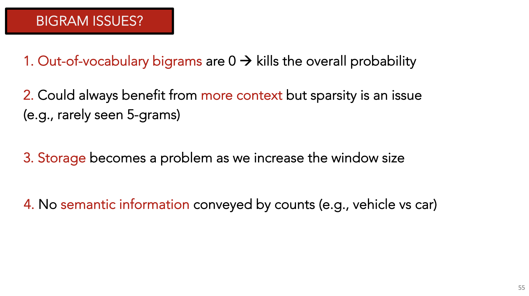
OOV: “Out of vocabulary” words, replace with <UNK>
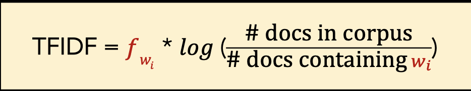
TF-IDF
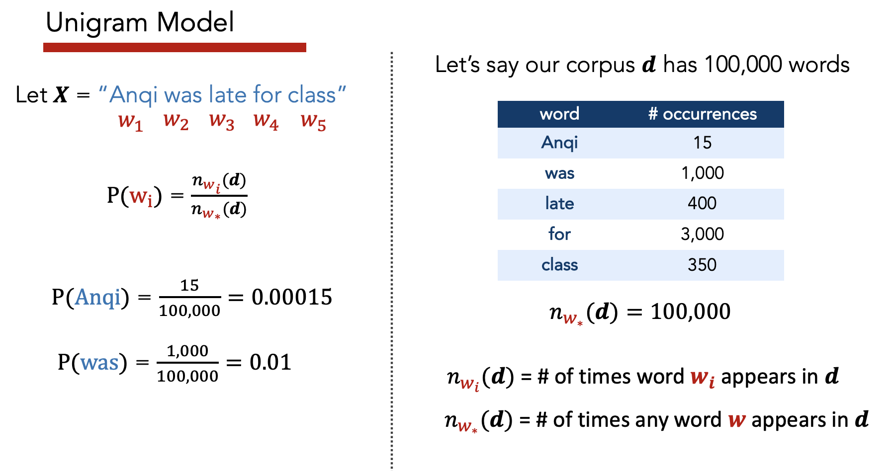
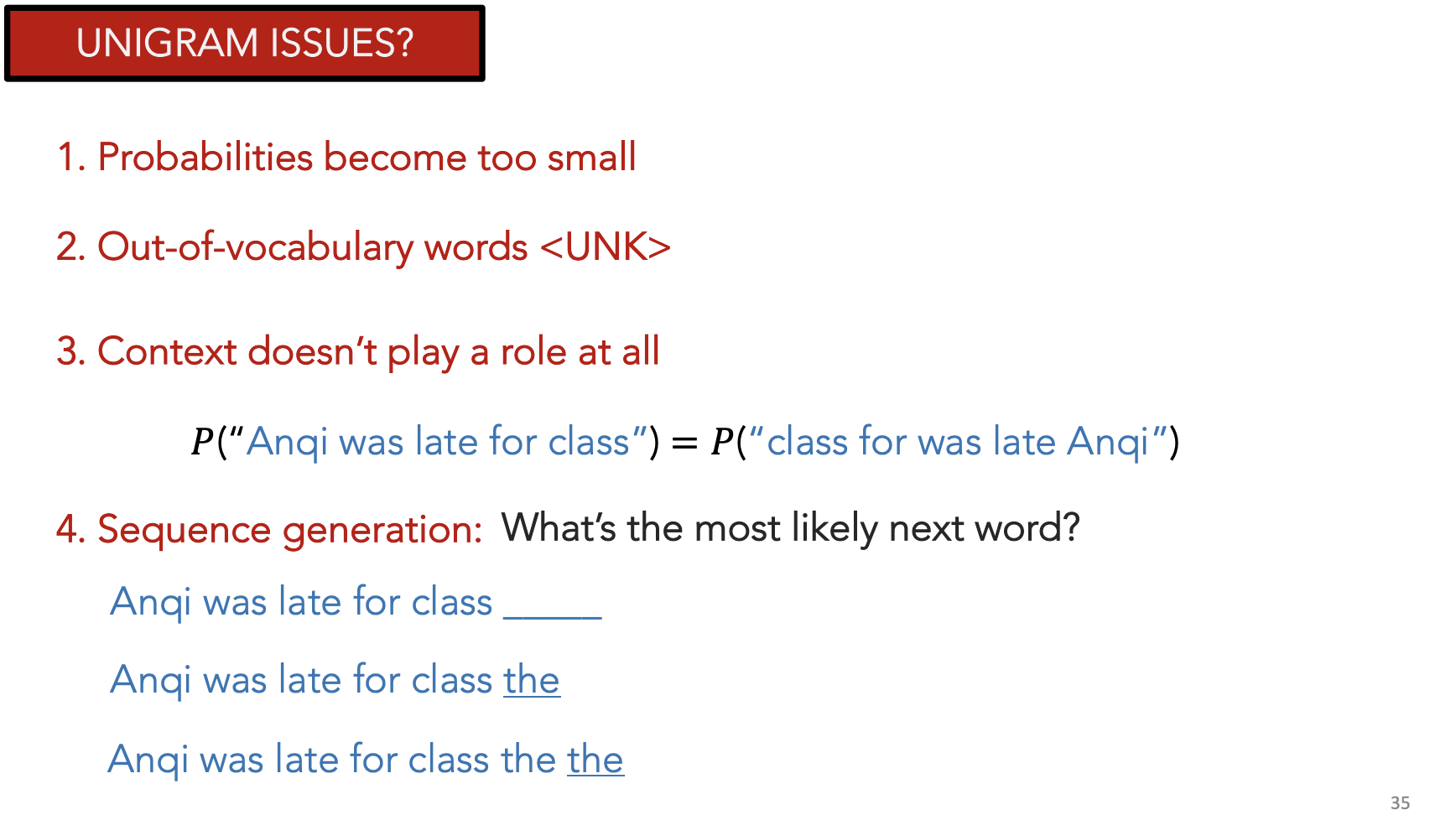
Unigram
Assume each 1-gram is independent.
\(P(w_1,...,w_T) = \prod_{t = 1}^T P(w_t)\)
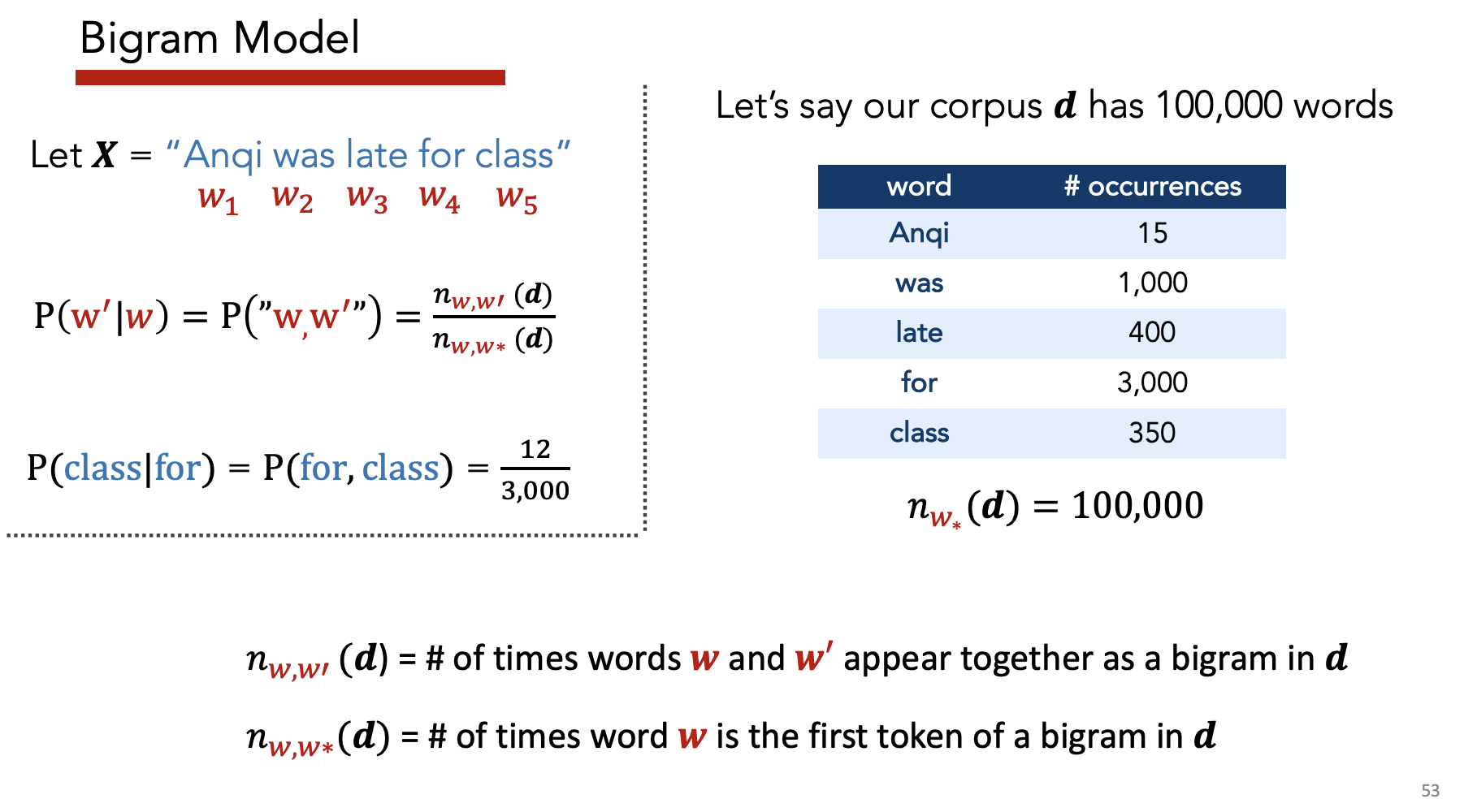
Bigrams
Assume each 2-gram is independent \(P(w_1,...,w_T) = \prod_{t = 2}^T P(w_t | w_{t-1})\)
N-Gram Model
Condition on all previous words in document \(P(w_1,...,w_T) = \prod_{t = 1}^T P(x_t | x_{t-1},...,x_1)\)
Evaluation
Entropy
- Interpretation: Avg number of bits needed to represent a word
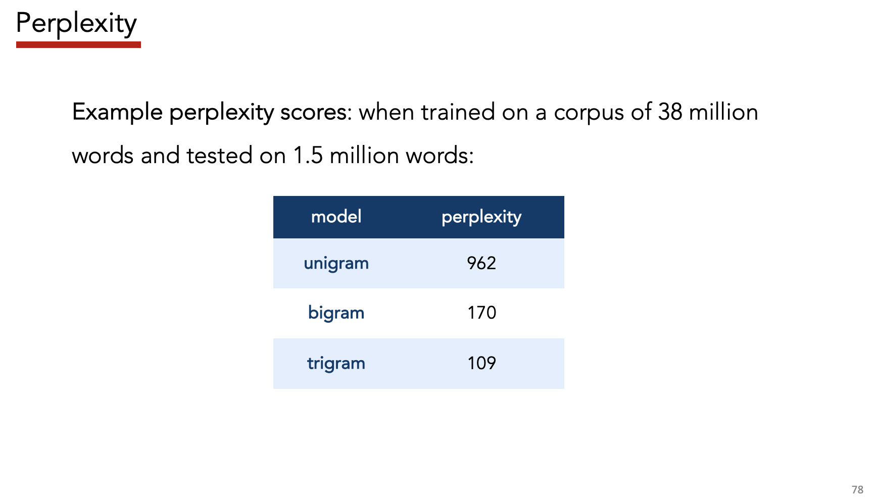
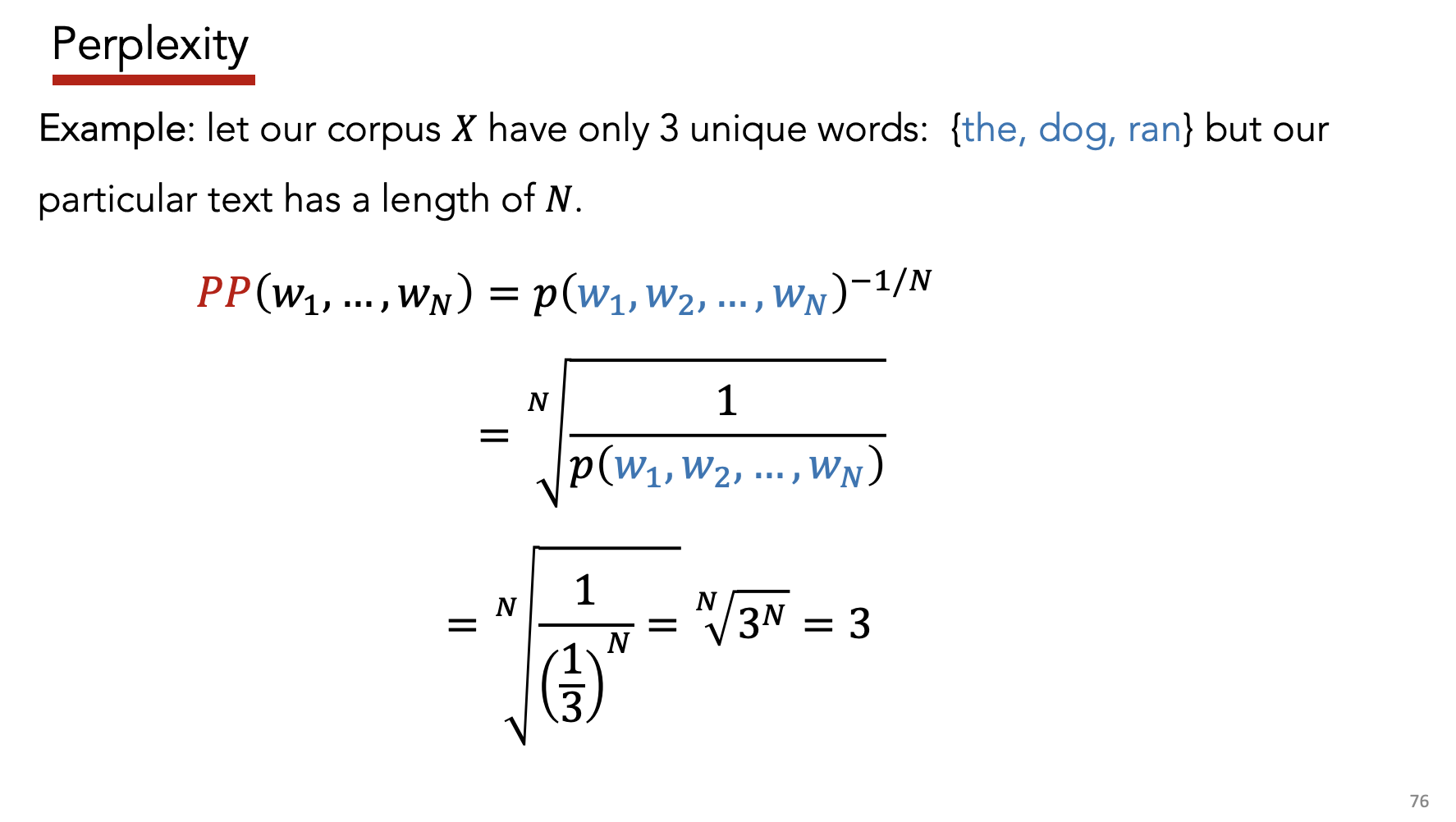
Perplexity
- Definition: Inverse probability of test set, normalized by number of words
- Aka: “exponentiated, per-word cross-entropy”
- Interpretation: Branching factor needed to predict next word – more branches = more uncertainty
- Good models have $PP \in [40, 100]$
-
If model assumes uniform distribution of words, then $PP = V $
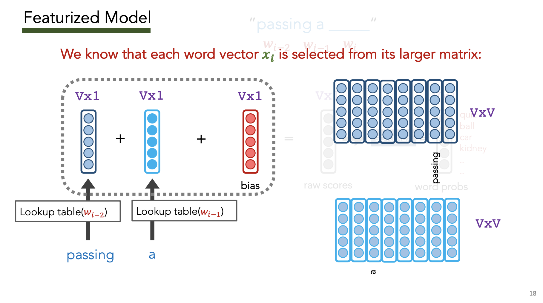
Featurized Model
| Goal: Have $# features « | V | $ |
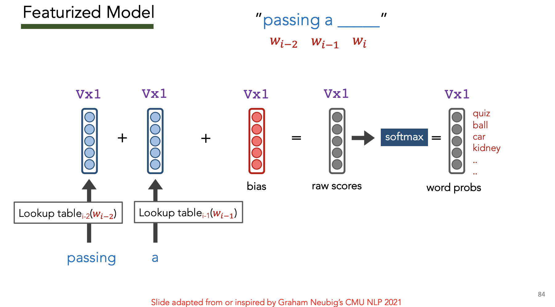
Goal: Learn embedding $v_i$ for each word $w_i$ i.e. learn the red bias vector and blue matrix $N\times V$
4) Neural Nets [Source]
Terms
Distributional: Meaning of word is determined by its context, i.e. “You shall know a word by the company it keeps”
Distributional Representation: Dense embedding vectors convey meaning of token by factoring in context
- Word Embedding (“Type-based”): **Distributional representation unique for each **word type, i.e. all “banks” have the same learned vector
- Examples: Bengio 2003, Word2Vec
- Contextualized Embedding (“Token-based”): Distributional representation unique for each token, i.e. the word “banks” can have different vectors depending on where it is used in the document
- Examples: RNNs, LSTMs, ELMo
Autoregressive LM: Predict next word only using previous words (previous outputs become inputs)
- e.g. I want a _____
- Evaluation: Perplexity
Masked LM: Predict “masked” word in middle of sequence using before/after words
- e.g. I want to _____ a bagel.
- Evaluation: Downstream NLP tasks which use learned embeddings
Bengio (2003)
Idea: Simultaneously learn representations + do modeling
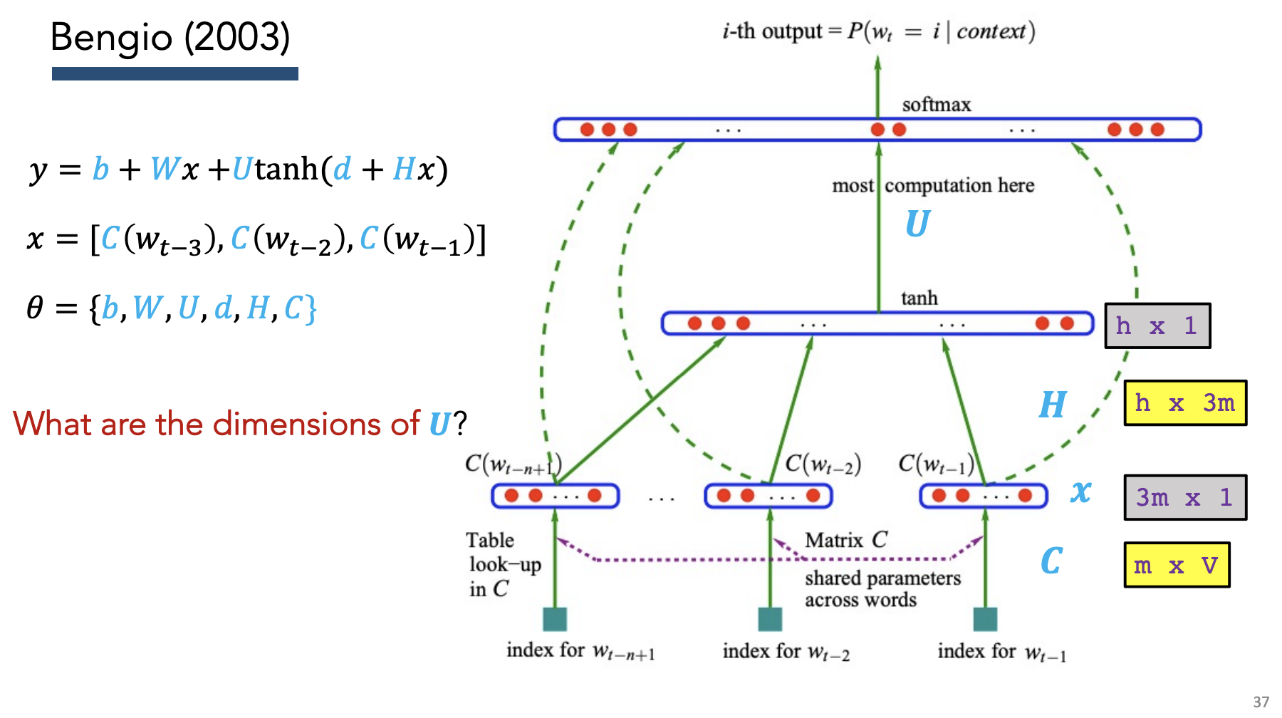
Training:
- Use weight matrix + bias to calculate probability of label
- Calculate CE loss
- Backprop to calculate gradients
- Update weight matrix + bias
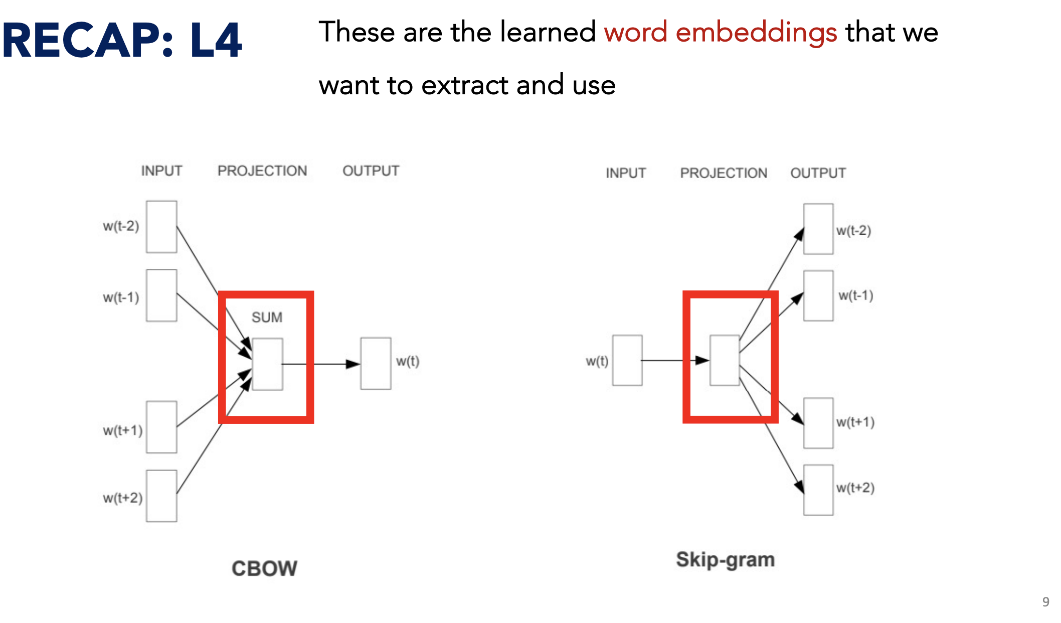
Word2Vec (2013)
Goal: Create word embeddings such that words with the same context have identical embeddings
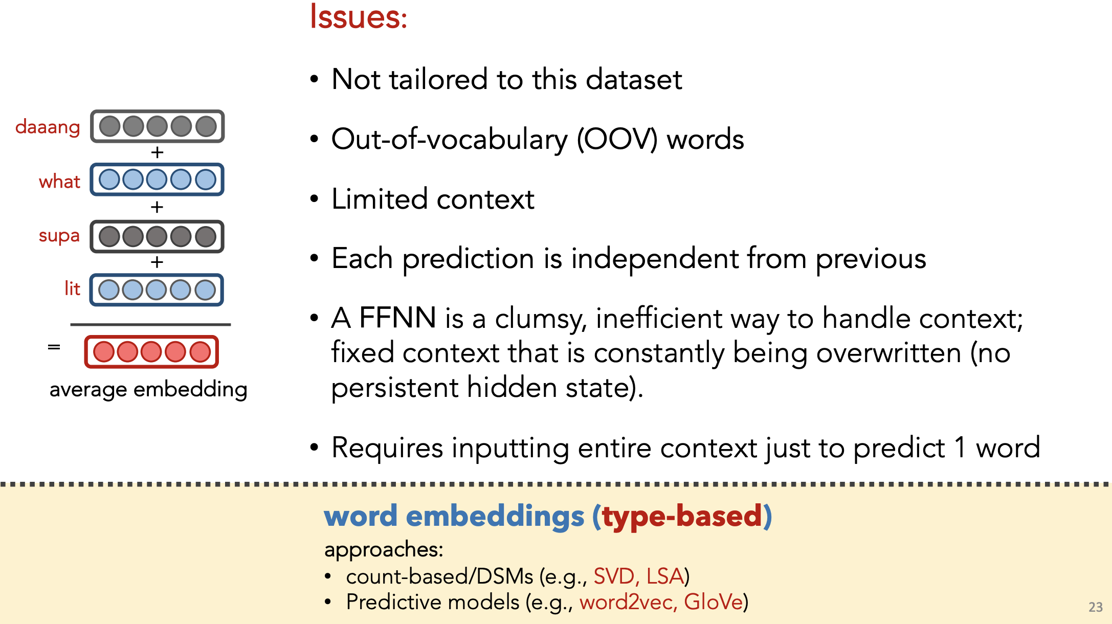
Approach 1) Continuous Bag-of-Words (CBOW)
Goal: Predict current word based on surrounding words
Algo:
- Iterate over corpus using sliding “context window” of size $N$, step size 1
- Use $2N$ context words (except for word at center of window) to predict center word
- Apply softmax, calculate loss
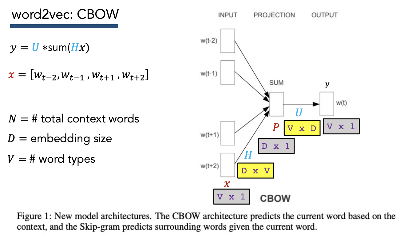 \(\begin{align*}
Hx &= (D \times V)(V \times 2N)\\
&= D \times 2N\\
sum(Hx) &= \text{row-wise sum across each index in the feature vector for each context word}\\
&= D \times 1\\
U * sum(Hx) &= (V \times D) (D \times 1)\\
&= V \times 1\\
y &= V \times 1
\end{align*}\)
\(\begin{align*}
Hx &= (D \times V)(V \times 2N)\\
&= D \times 2N\\
sum(Hx) &= \text{row-wise sum across each index in the feature vector for each context word}\\
&= D \times 1\\
U * sum(Hx) &= (V \times D) (D \times 1)\\
&= V \times 1\\
y &= V \times 1
\end{align*}\)
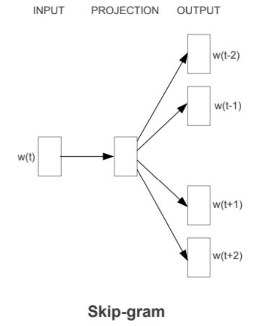
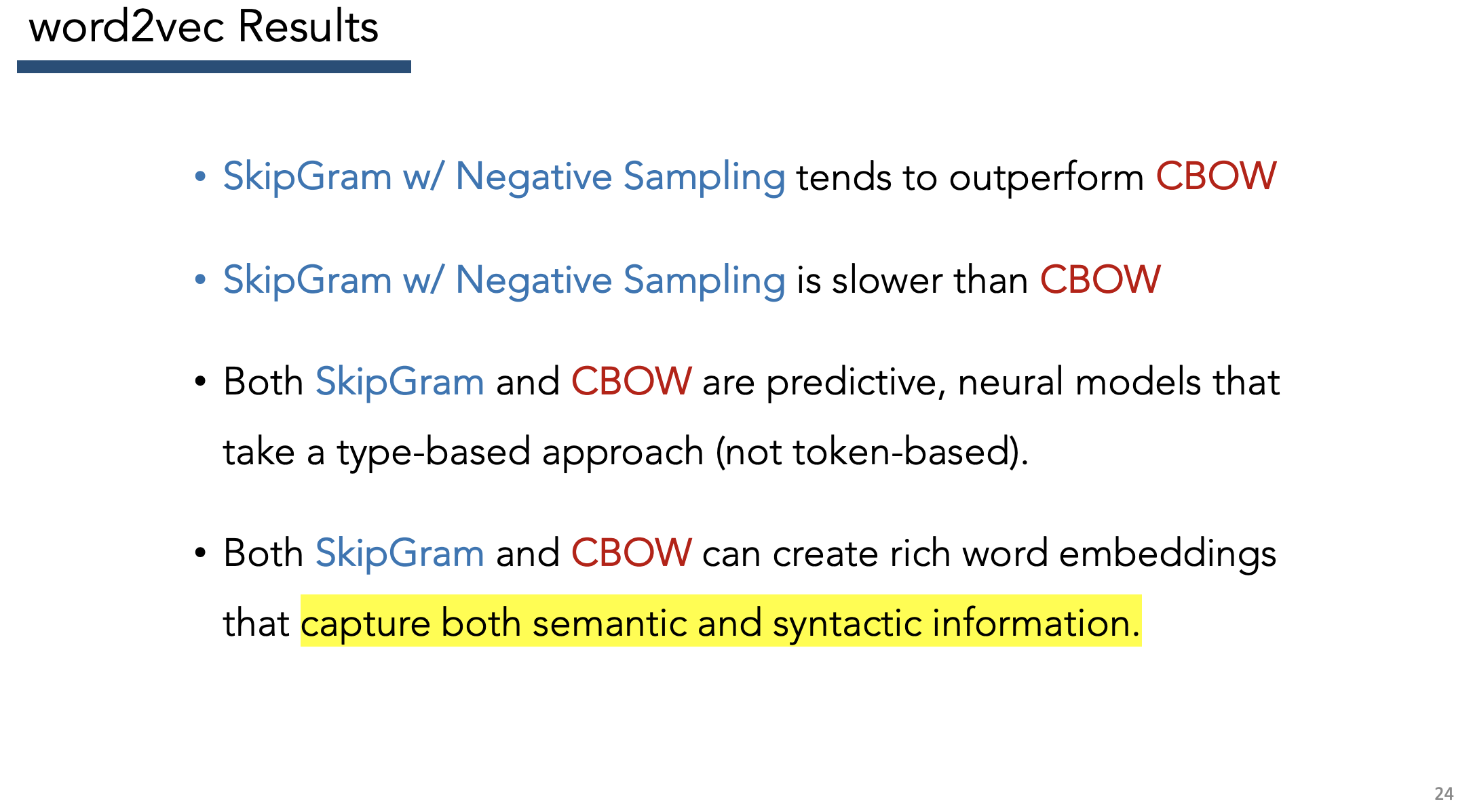
Approach 2) Skip-gram + negative sampling
Goal: Predict surrounding words given current word
Algo:
- Iterate over corpus using sliding “context window” of size $N$, step size 1
- Use center word to predict all $2N$ context words
- Apply softmax, calculate loss
Need to add negative samples, otherwise model will simply learn to predict 1.
General Word2Vec Takeaways
Interpretation:
- Smaller window size -> similar embeddings means “interchangeable” words
- Larger window size -> similar embeddings means “related” words
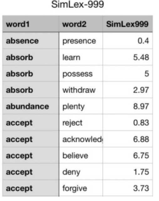
Evaluation
Word similarity
Use SimLex-999 dataset to compare embedding distance with word similarity
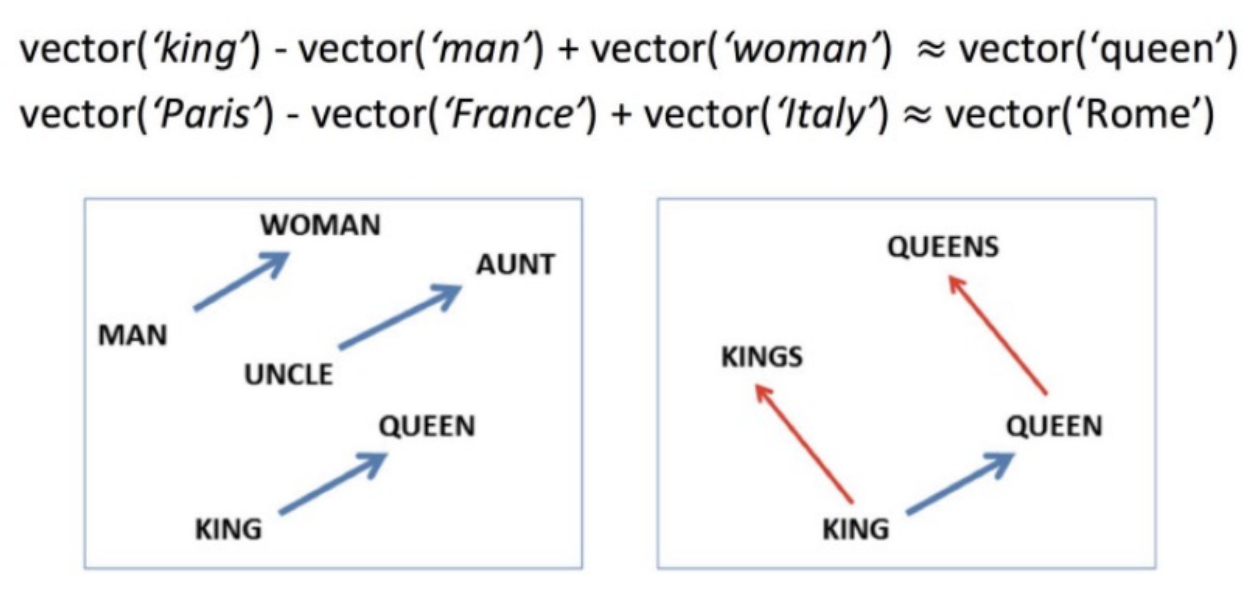
Word analogy
Check whether analogies hold in embedding space
Downstream NLP tasks
“External” to model to evaluate utility of embeddings
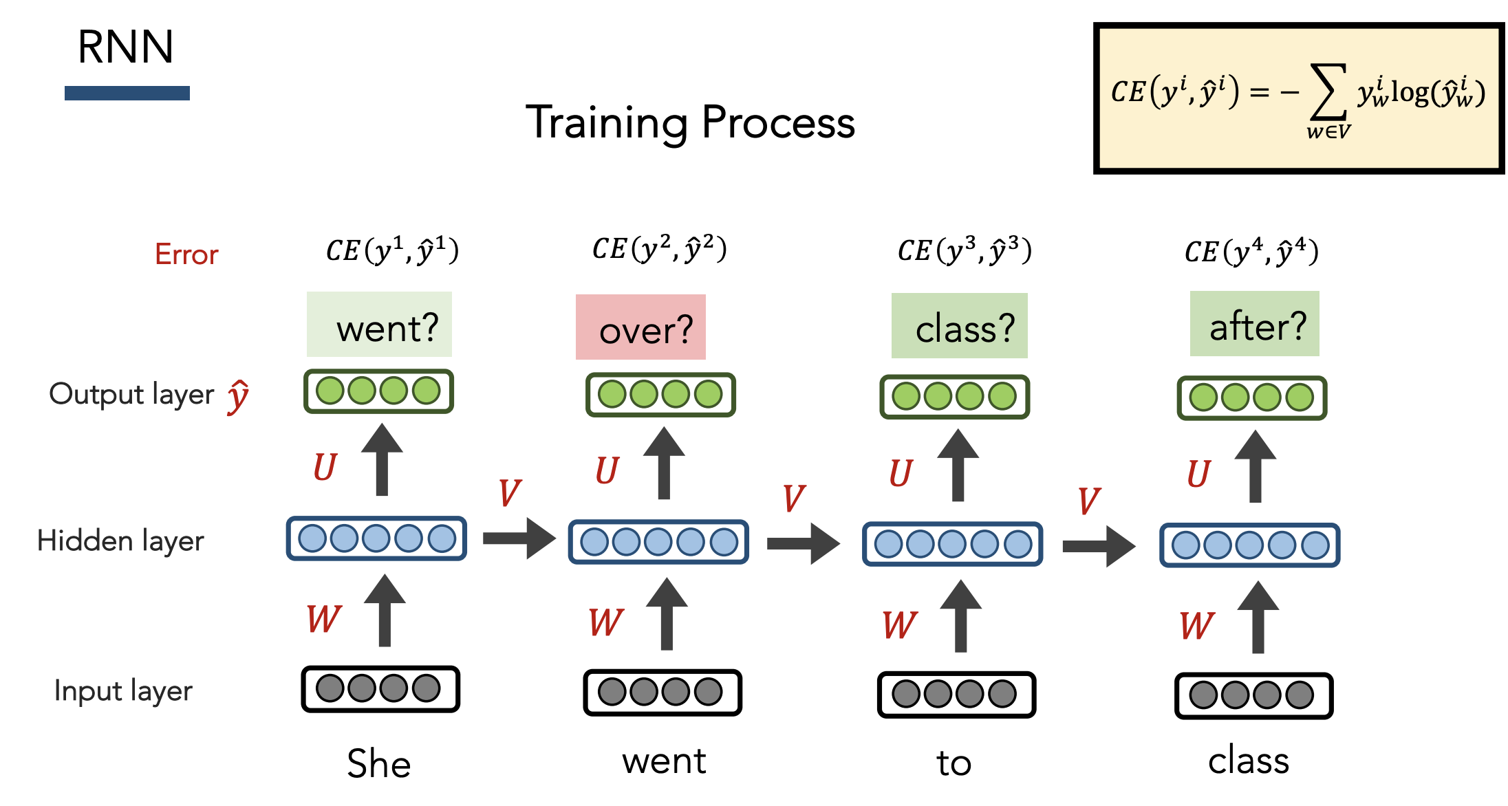
5) RNNs [Source]
Definition: NN with a non-linear combination of recurrent state (i.e. “hidden layer”) and the input
Goal: Model long-range dependencies in language (i.e. have “infinite” concept of past words, as opposed to fixed window used by Word2Vec)
Idea: Re-use hidden layer from previous output to predict next output
Hidden layer represents the “meaning” of a word
Training
- Regardless of output predictions, feed in the actual ground truth inputs at each step (i.e. not autoregressive)
- Total loss = avg across all words
Alternative view of the same RNN model: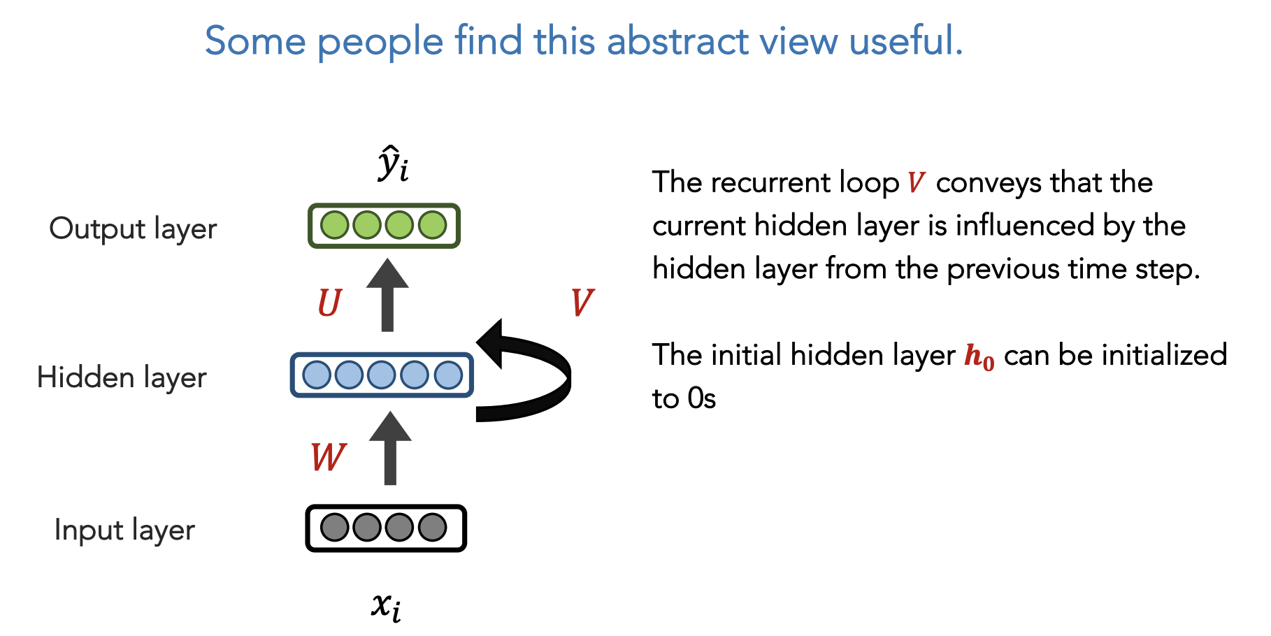
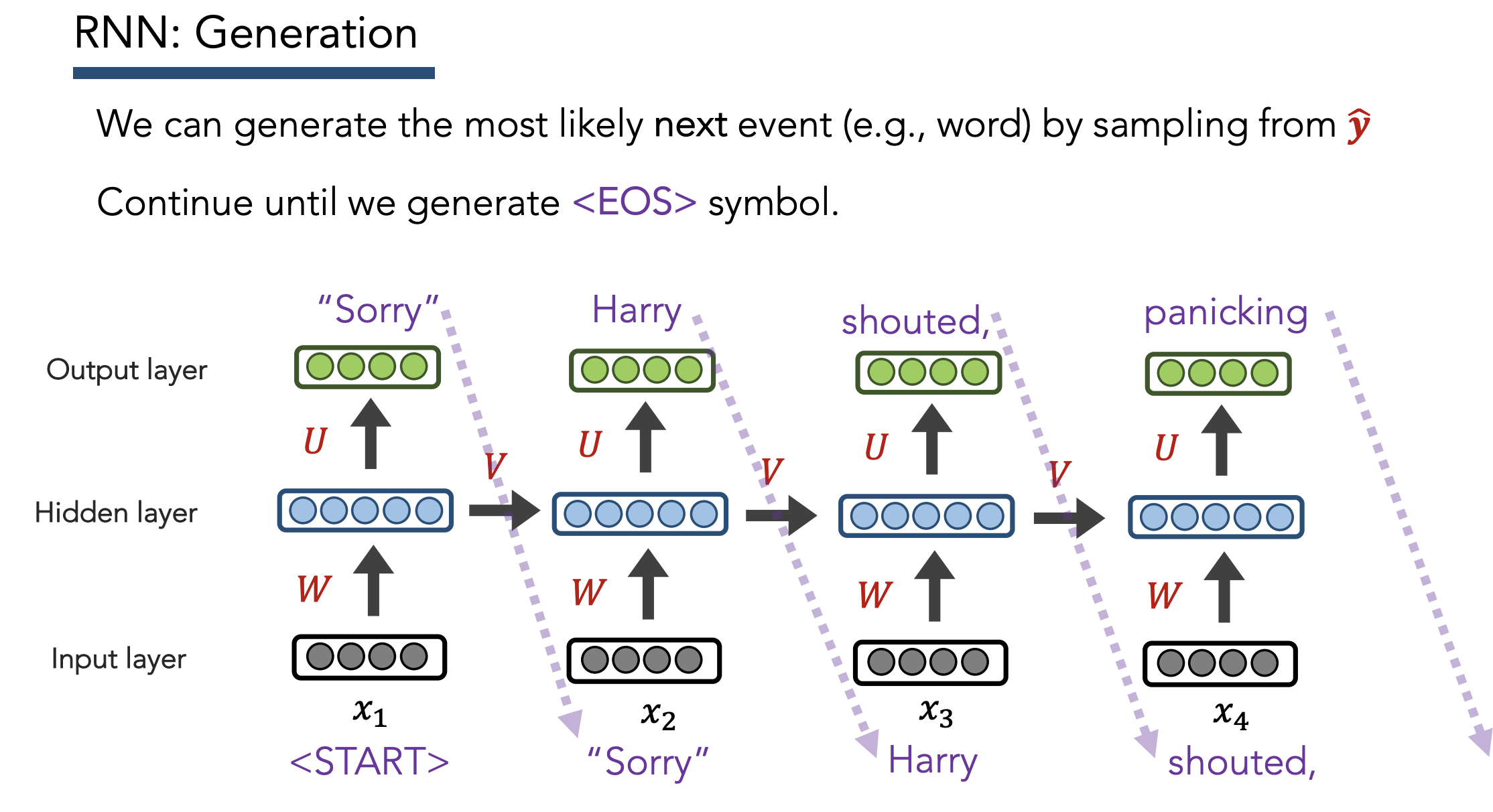
Testing
- Feed previous output as input to next output
- NOTE: Same word (“Harry”) can yield different most probable outputs depending on context (thanks to hidden embedding, unlike vanilla NNs + n-grams)
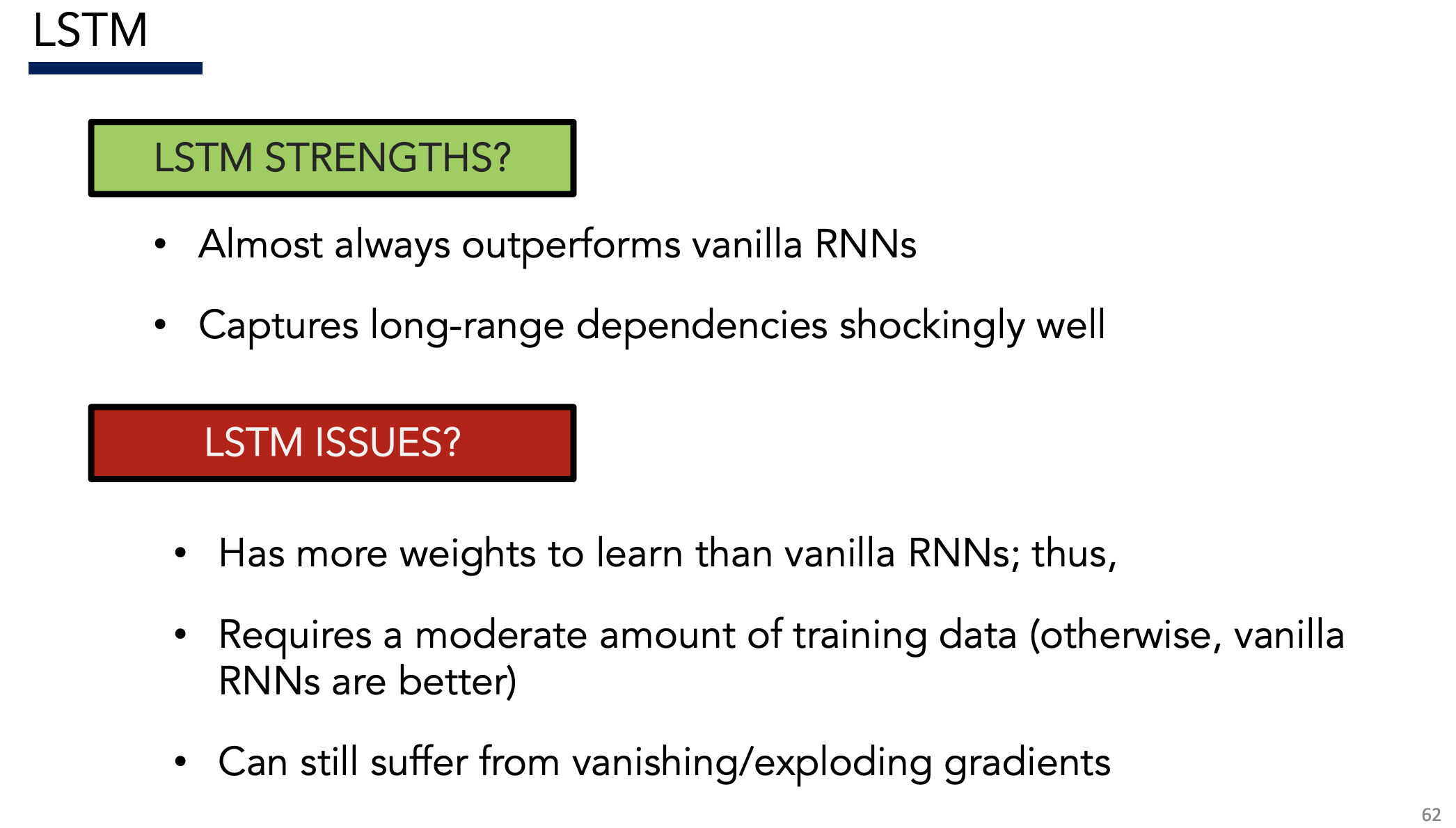
Strengths + Issues
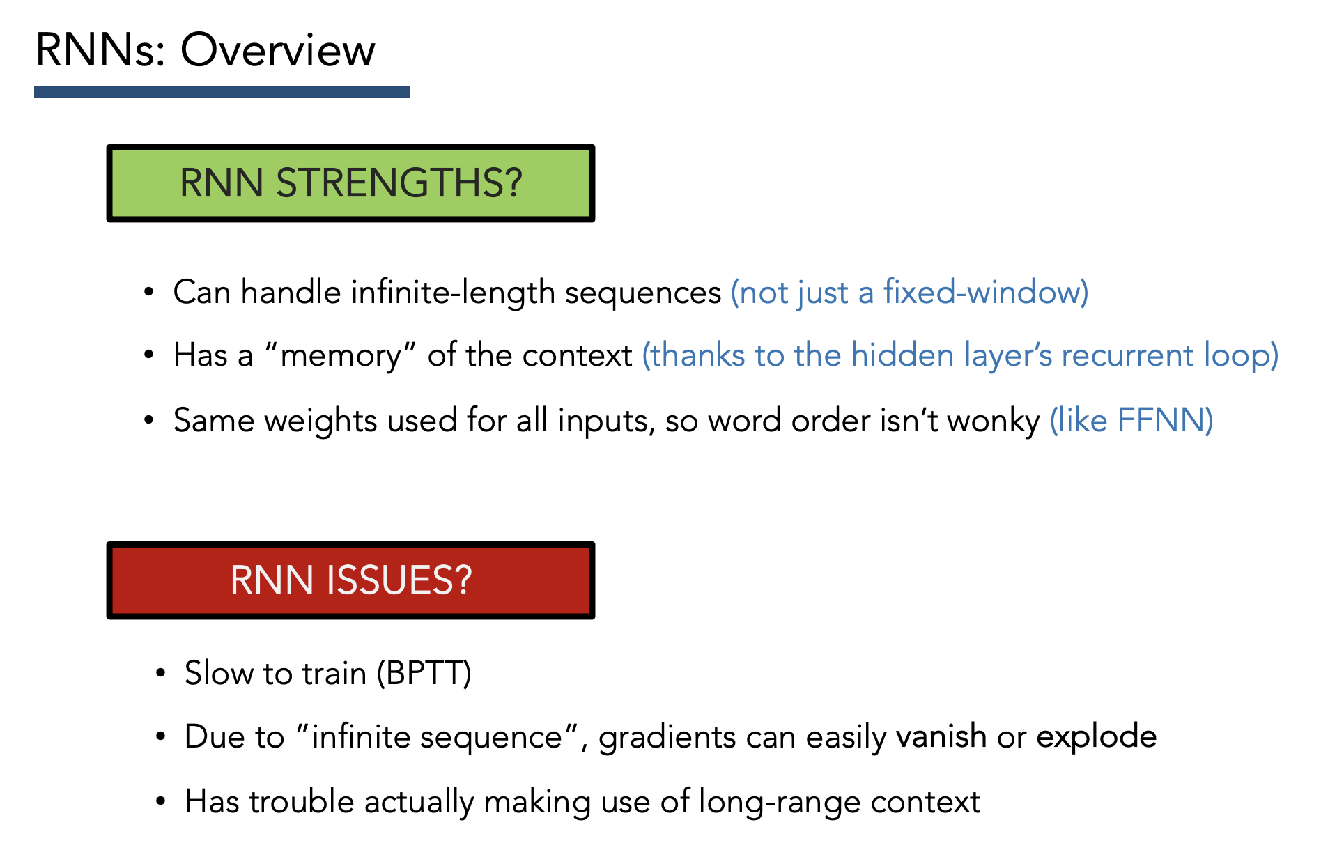
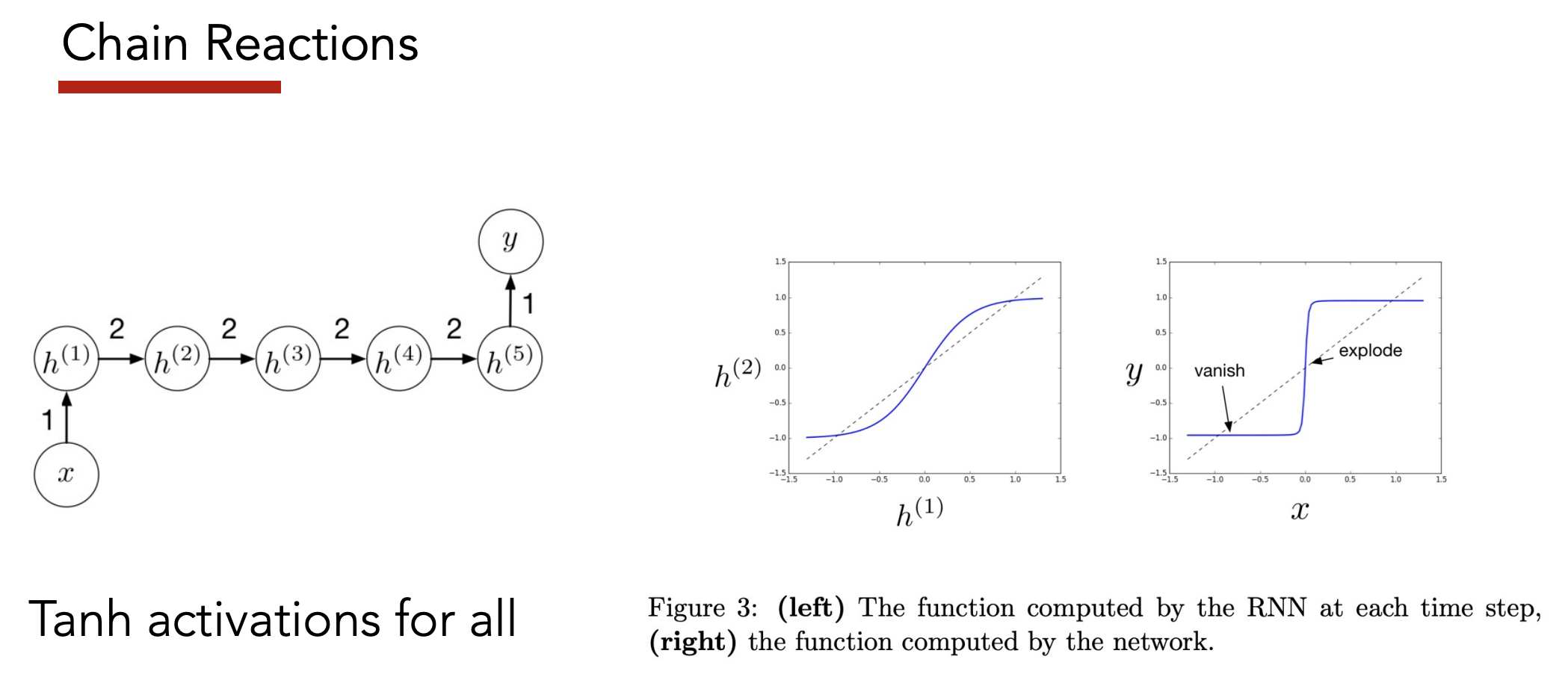
Issue: Exploding + Vanishing Gradients
Caused by taking chain rule of many time steps
-
Small gradient = far away context is “forgotten”
-
Large gradient = recency bias without context
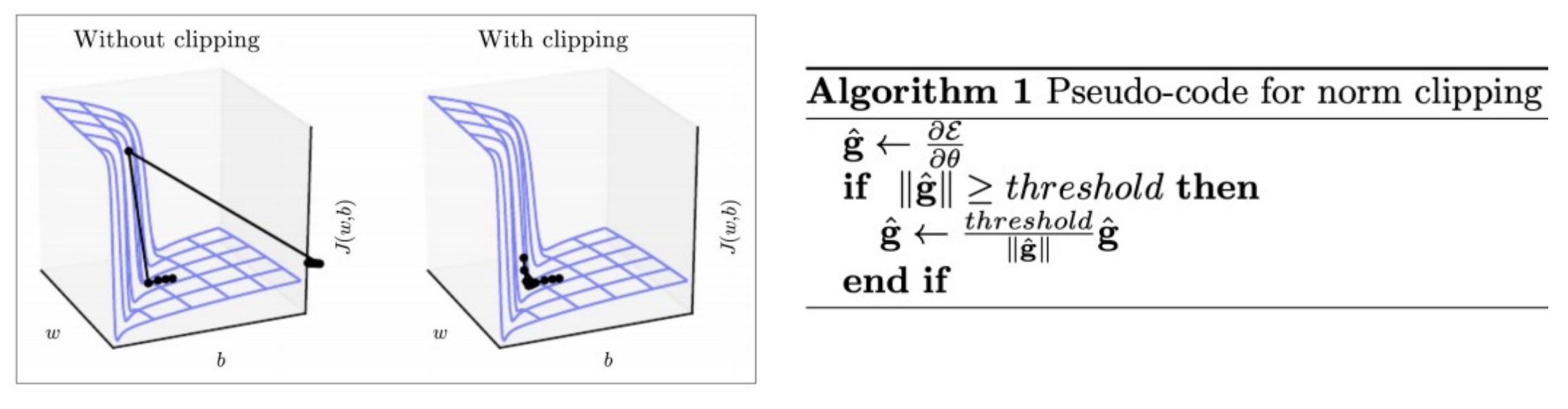
Solution: Gradient Clipping
Fixes the exploding gradients problem
- Sets max magnitude (i.e. “norm”) of gradient to some threshold
- Helps with numerical stability of training
- Doesn’t make model more accurate
6) LSTMs [Source]
Idea: Better RNN by fixing long-term forgetting issue
Solution: Add a dedicated memory cell $C$ for long-term memory, in addition to the usual hidden state $h$
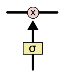
Modify $C$ via three gates:
- Forget
- Input
Each gate looks like this in diagrams:
Overview
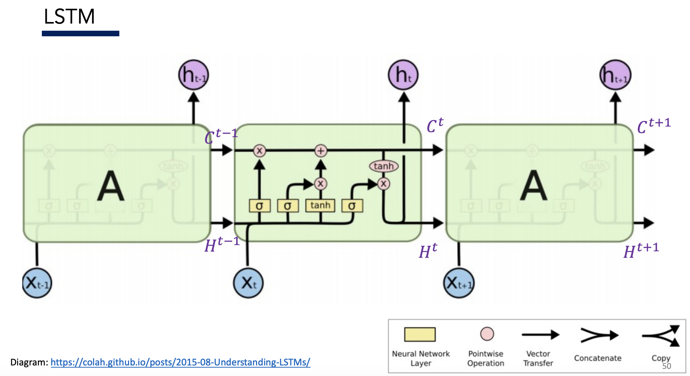
Images in below sections are taken from: https://colah.github.io/posts/2015-08-Understanding-LSTMs/
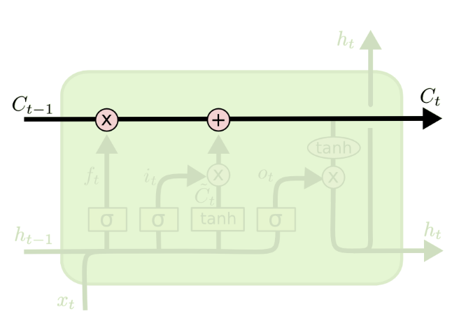
Cell State
Cell state $C$ is a “conveyor belt” – it runs through the LSTM and gets modified by $x$ and $h$
Gates
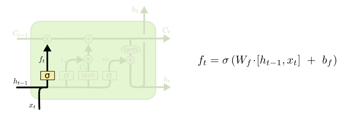
1) Forget Gate
- Goal: Decide what info to throw out from $C_{t-1}$, based on $h_{t-1}$ and $x_t$
- Interpretation: Forget old memories
- $\sigma$ generates a value between $[0,1]$ for each element in $C_{t-1}$
- Value of 1 = “completely keep this element in long-term memory $C_{t-1}$”
- Value of 0 = “completely forget this element from long-term memory $C_{t-1}$”
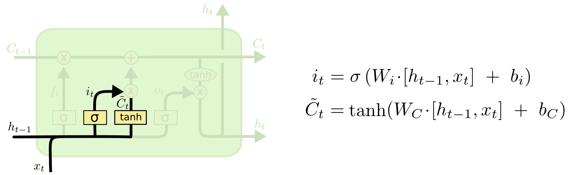
2) Input Gate
- Goal: Decide what info to change in $C_{t-1}$, based on $h_{t-1}$ and $x_t$
- Interpretation: Make new memories
- $\sigma$ generates a value between $[0,1]$ for each element in $C_{t-1}$ to decide which values to update
- $tanh$ squashes $h_{t-1}, x_t$ into new “candidate” values for $C_{t-1}$
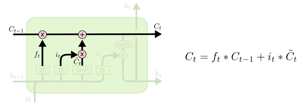
2b) Make Updates
Forget old memories: $f_t * C_{t-1}$
Update memory with new values (scaled by importance $i$): $i_t * \tilde{C}_t$
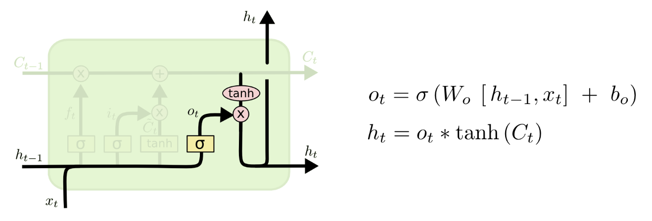
3) Output Gate
- Goal: Decide what to output, based on $C_t, h_{t-1}, x_t$
- Interpretation: Make new memories
- $\sigma$ generates a value between $[0,1]$ for each element in $C_{t-1}$ to decide which values of cell state go into new hidden state $h_t$
- $tanh$ squashes $C_t$ into new hidden state values $h_t$
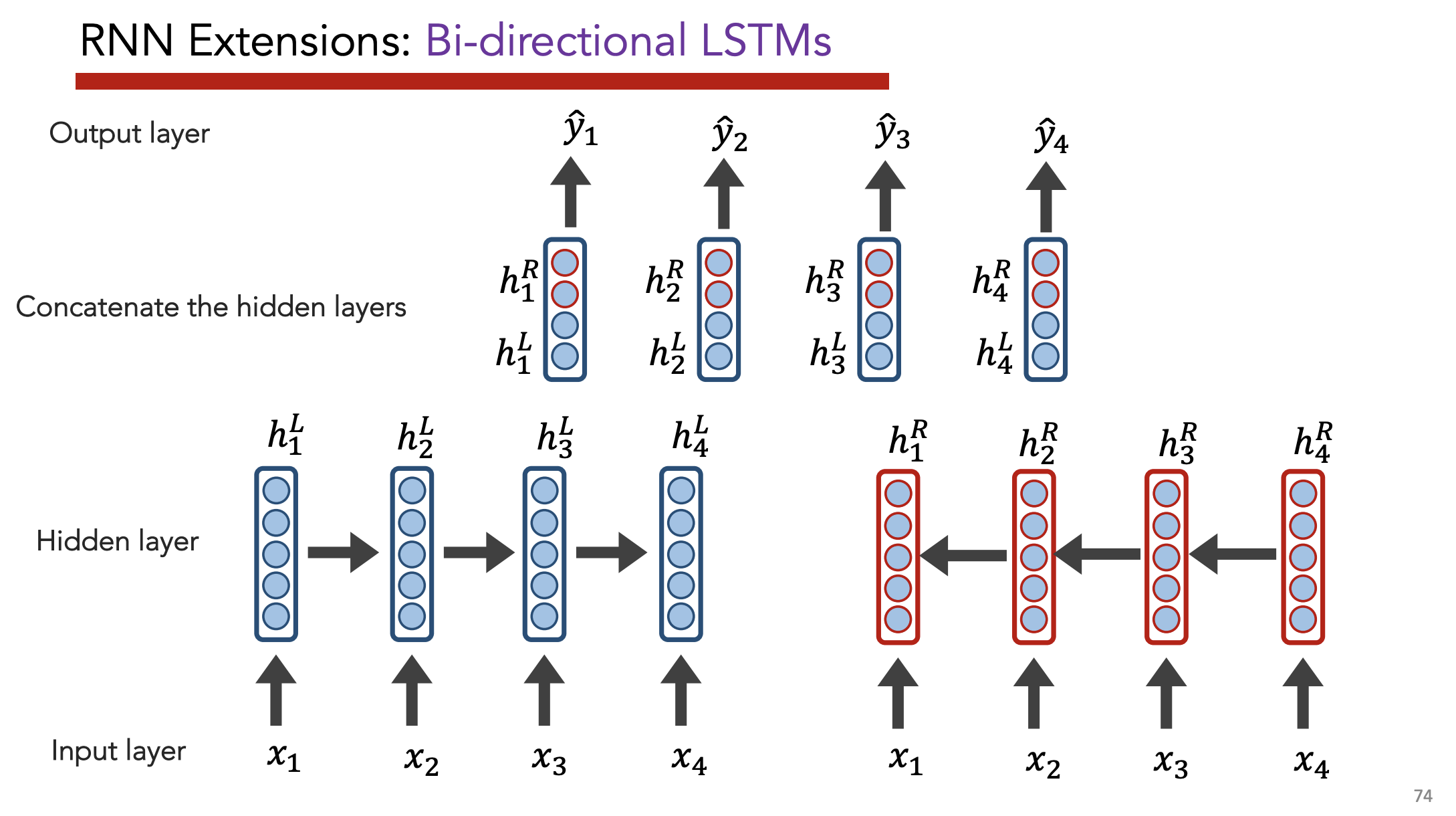
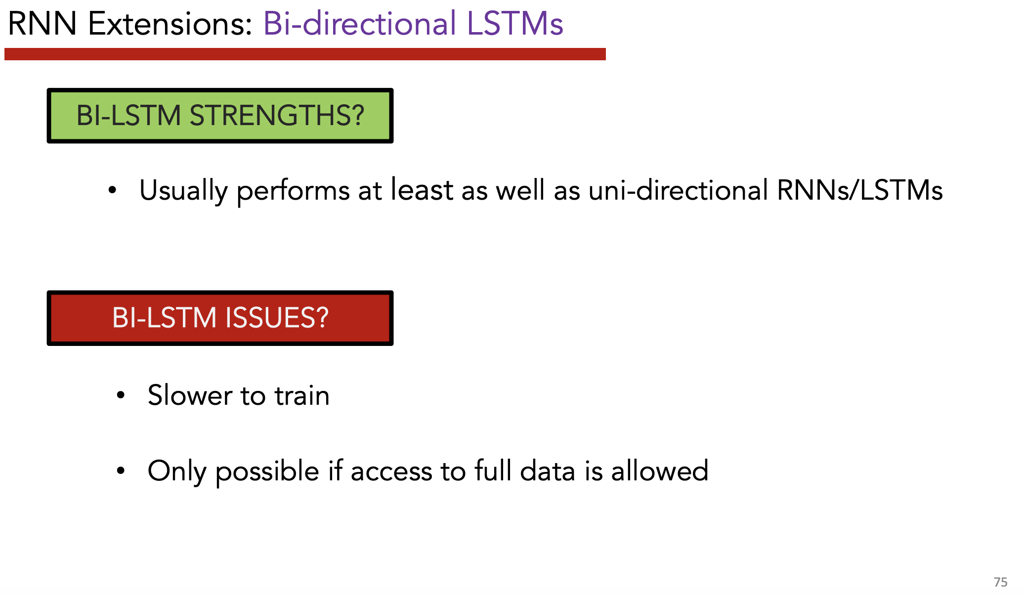
Bi-Directional LSTMs
If full text is available at test time, then use context in both left-to-right and right-to-left directions
Stacked LSTMs
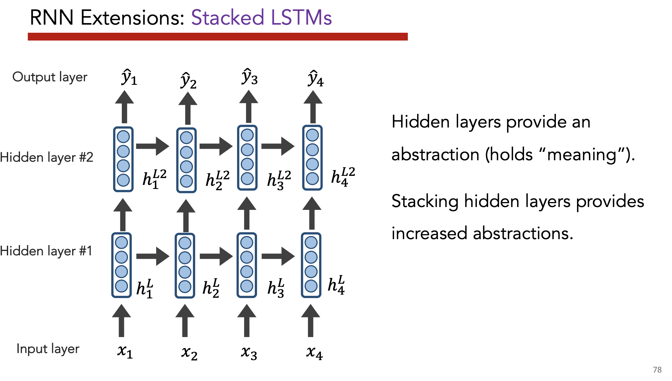
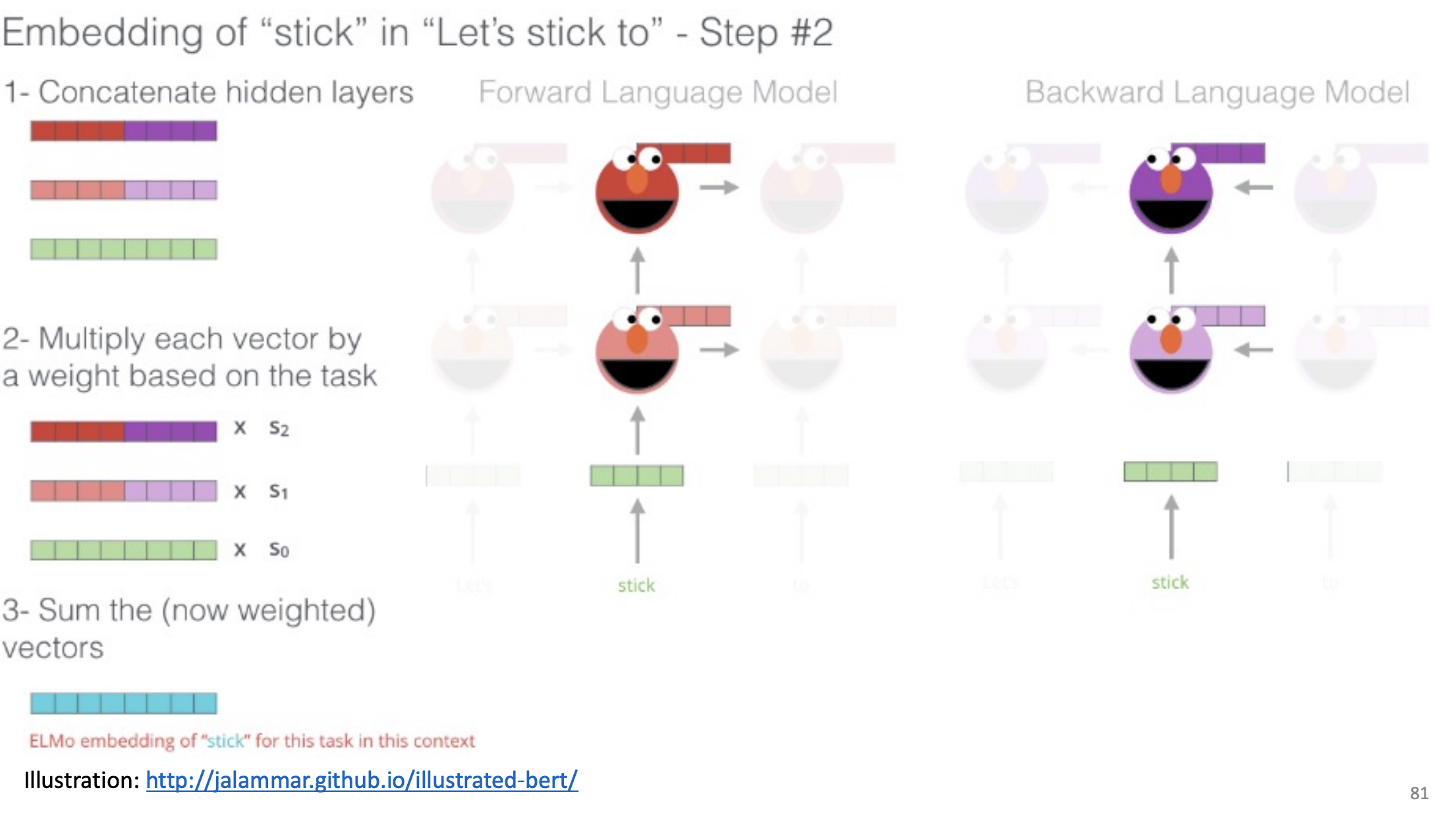
ELMo = Stacked, Bi-directional LSTM
- Yields “incredibly good contextualized embeddings”
Overview
7) Sequence Generation [Source]
Types of prediction
| Input | Output | |
|---|---|---|
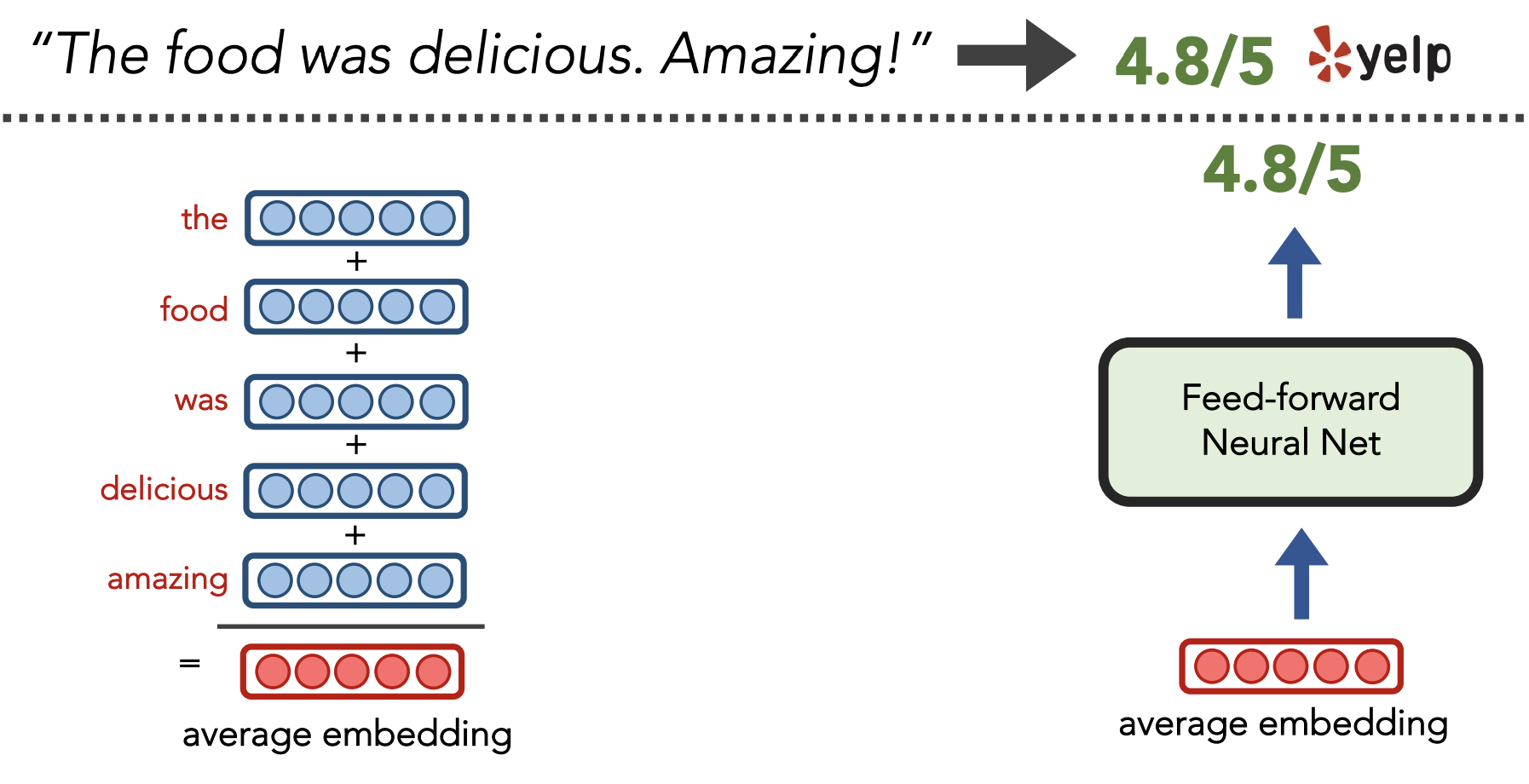
| Regression | I love hiking! | 0.9 |
| Binary classification | I love hiking! | + or - sentiment |
| Multi-class classification | I love hiking! | Category 1, 2, 3, 4, or 5 |
| Structured | I love hiking! | PRP VBP NN |
Unconditioned + Conditional Prediction
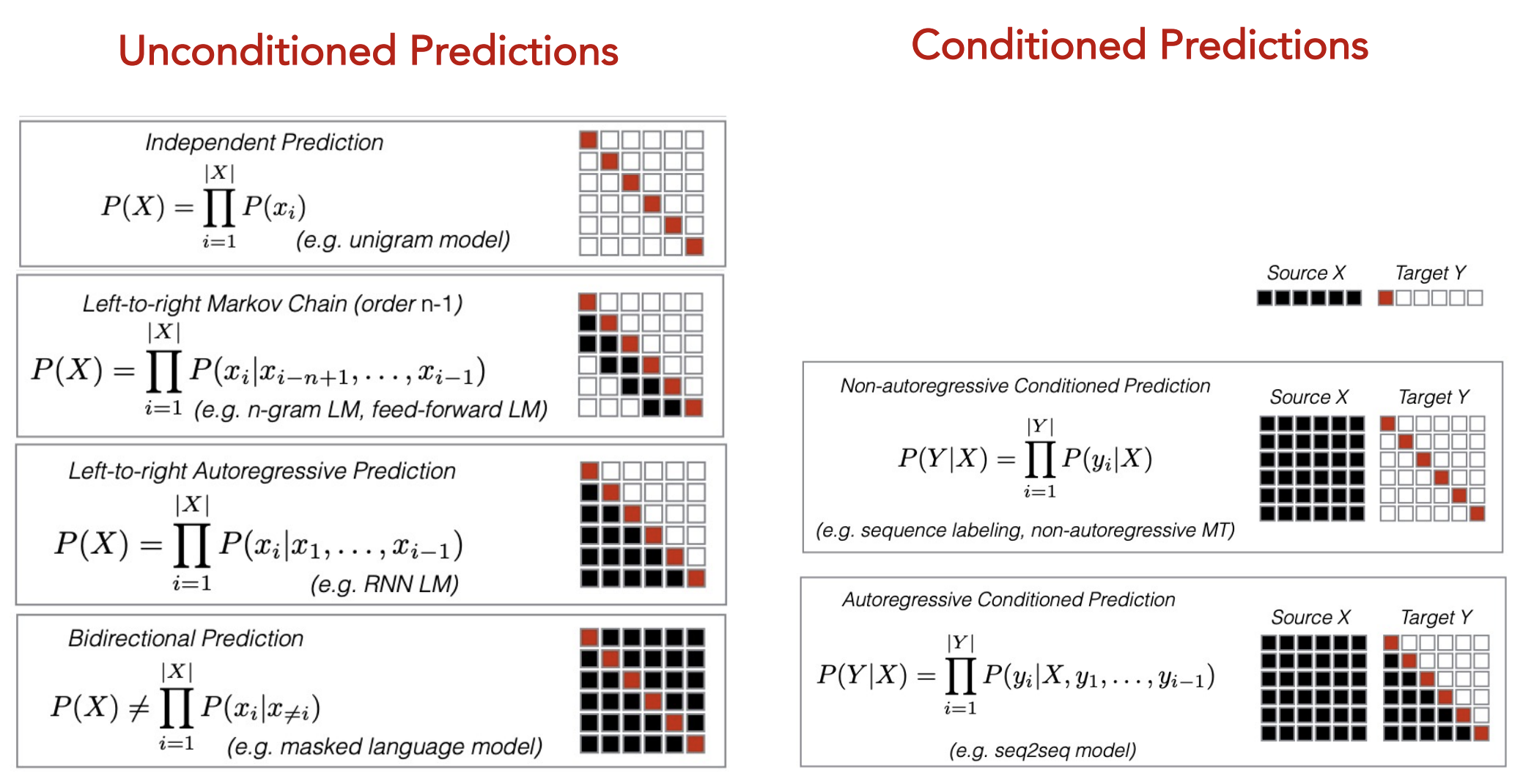
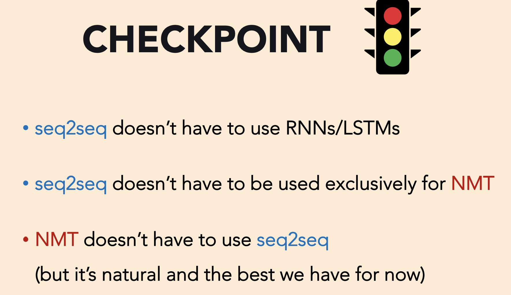
Seq2Seq Model
Problem: With LSTMs/RNNs, we can only have a fixed length output (either equal to the input sequence length or some fixed constant).
- We go from $N \rightarrow { 1, N }$
What if we want a variable length output? e.g. when translating between languages
- We want to go from $N \rightarrow M$
Solution: Treat “sequences” as the fundmanetal unit we work with
- Have two RNNs, one “encoder” and one “decoder” – “seq2seq” model
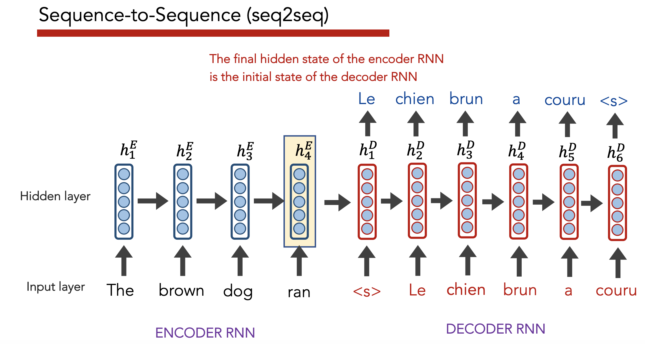
Training + Inference
Training: Backprop loss from decoder outputs all the way back to beginning (i.e. both encoder and decoder)
Testing: Run decoder until outputs <S> token. Each decoder output $\hat{y}i$ becomes subsequent input $x{i + 1}$
Strengths
- Main benefit of seq2seq = having a separate encoder/decoder allows outputs to be variable length
Attention
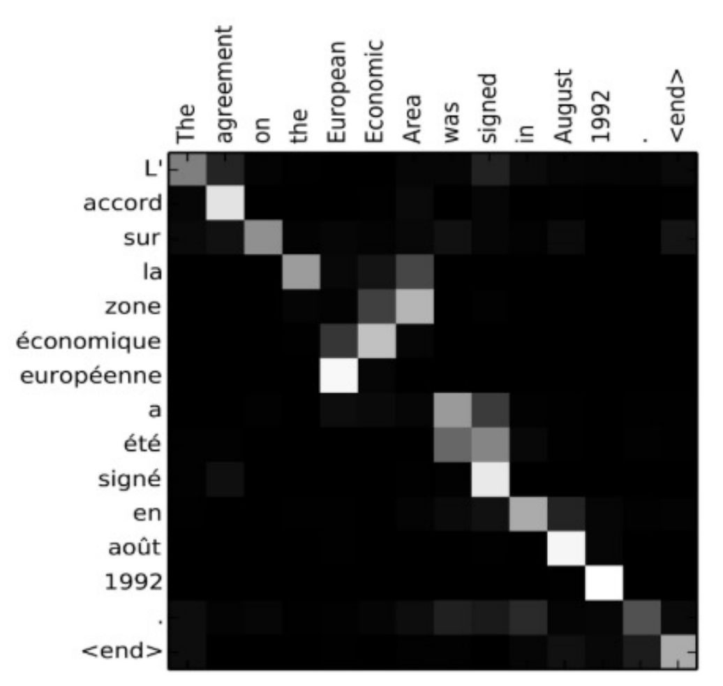
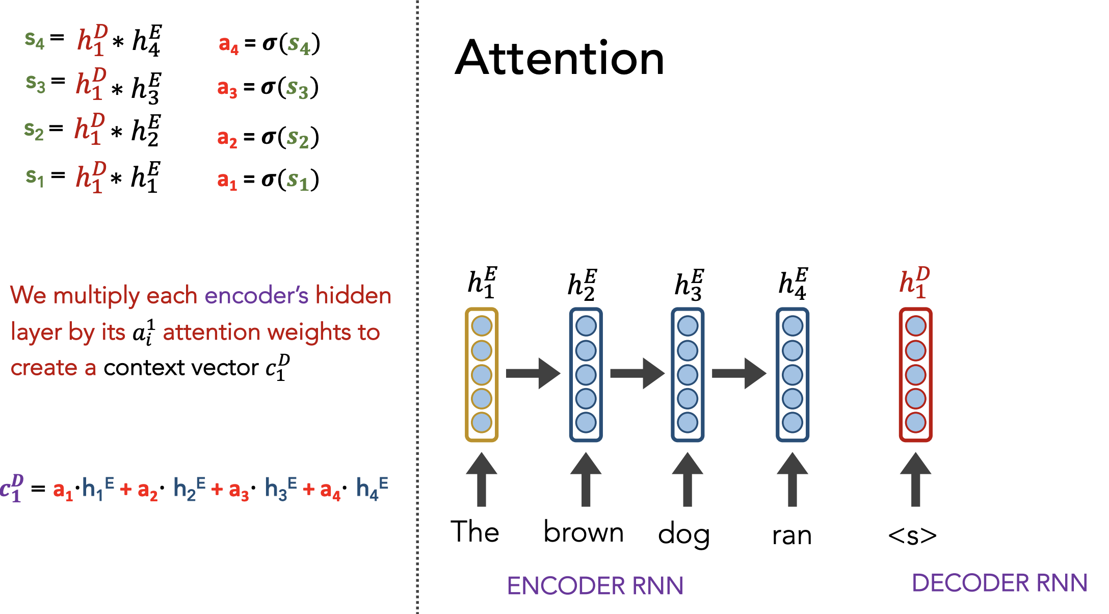
Insight: Instead of just paying attention to the last embedding, pay attention (weighted by importance) to all hidden states generated by the encoder as it reads the input sequence.
Definition: Attention allows a decoder, at each time step, to focus/use different amounts of the encoder’s hidden states
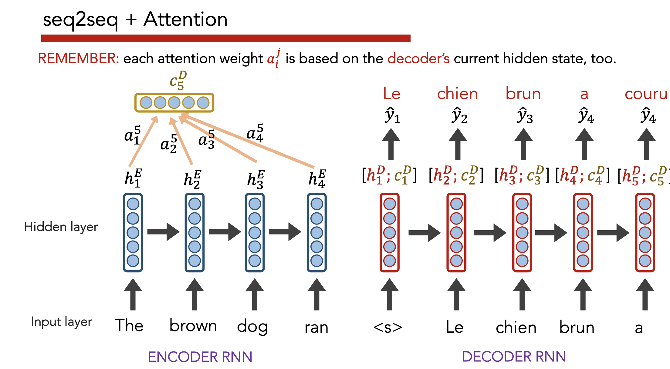
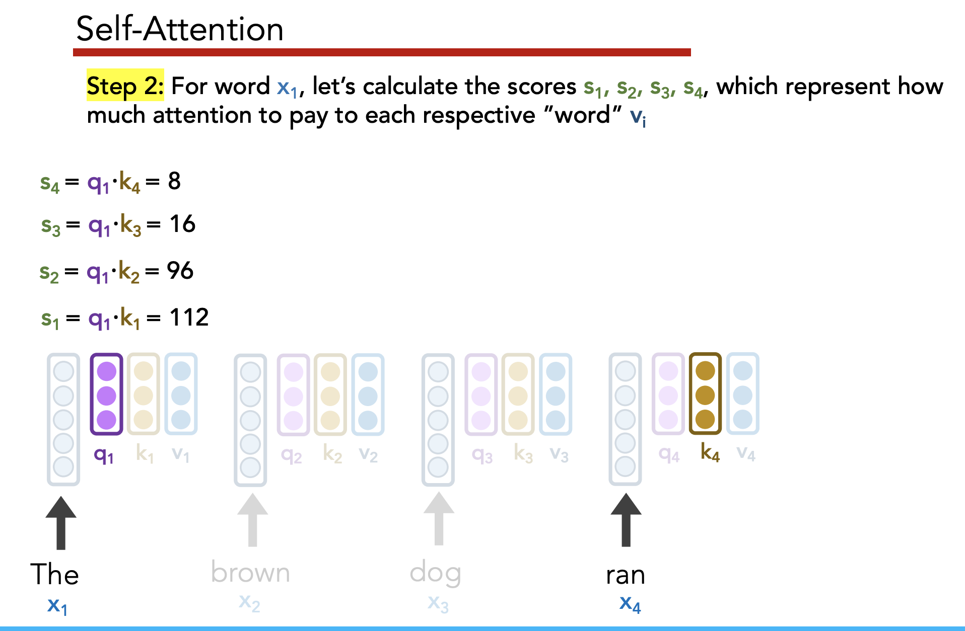
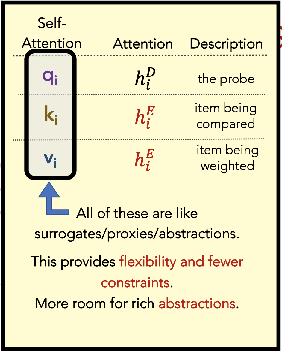
- Each hidden state $h_i^E$ gets a unique raw weight $e_i$ based on its relevance to the decoder state $h_j^D$. This raw weight is calculated via a separate NN (but can be calculated via any arbitrary function).
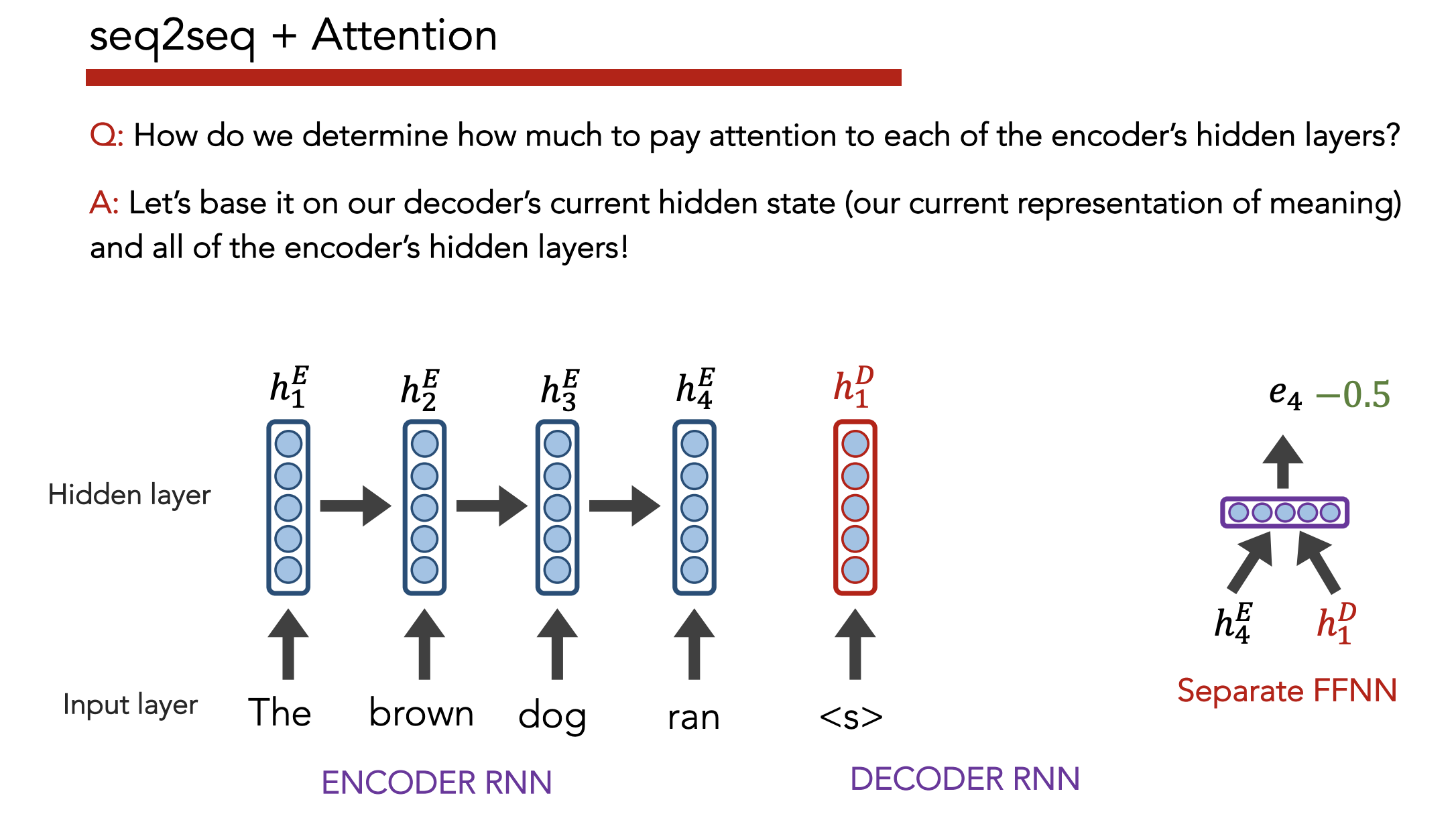
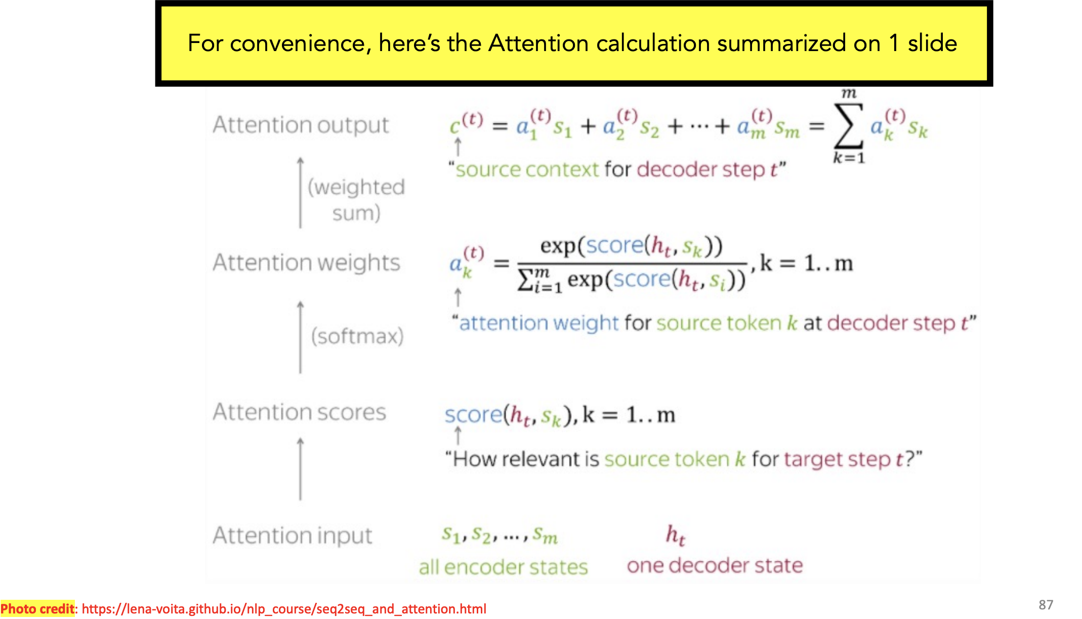
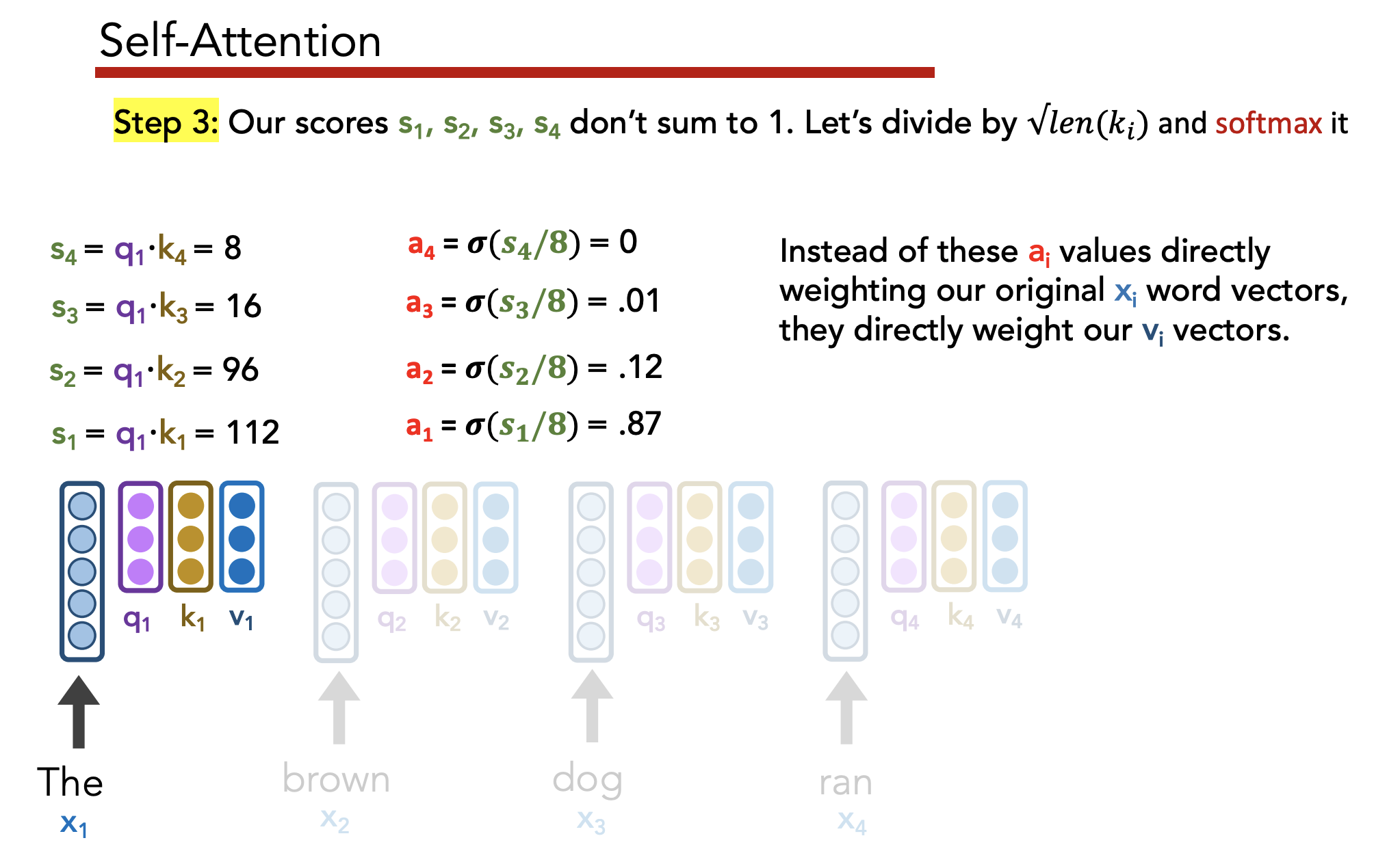
- Softmax across all $e_i$ to get an “attention score” $a_i$
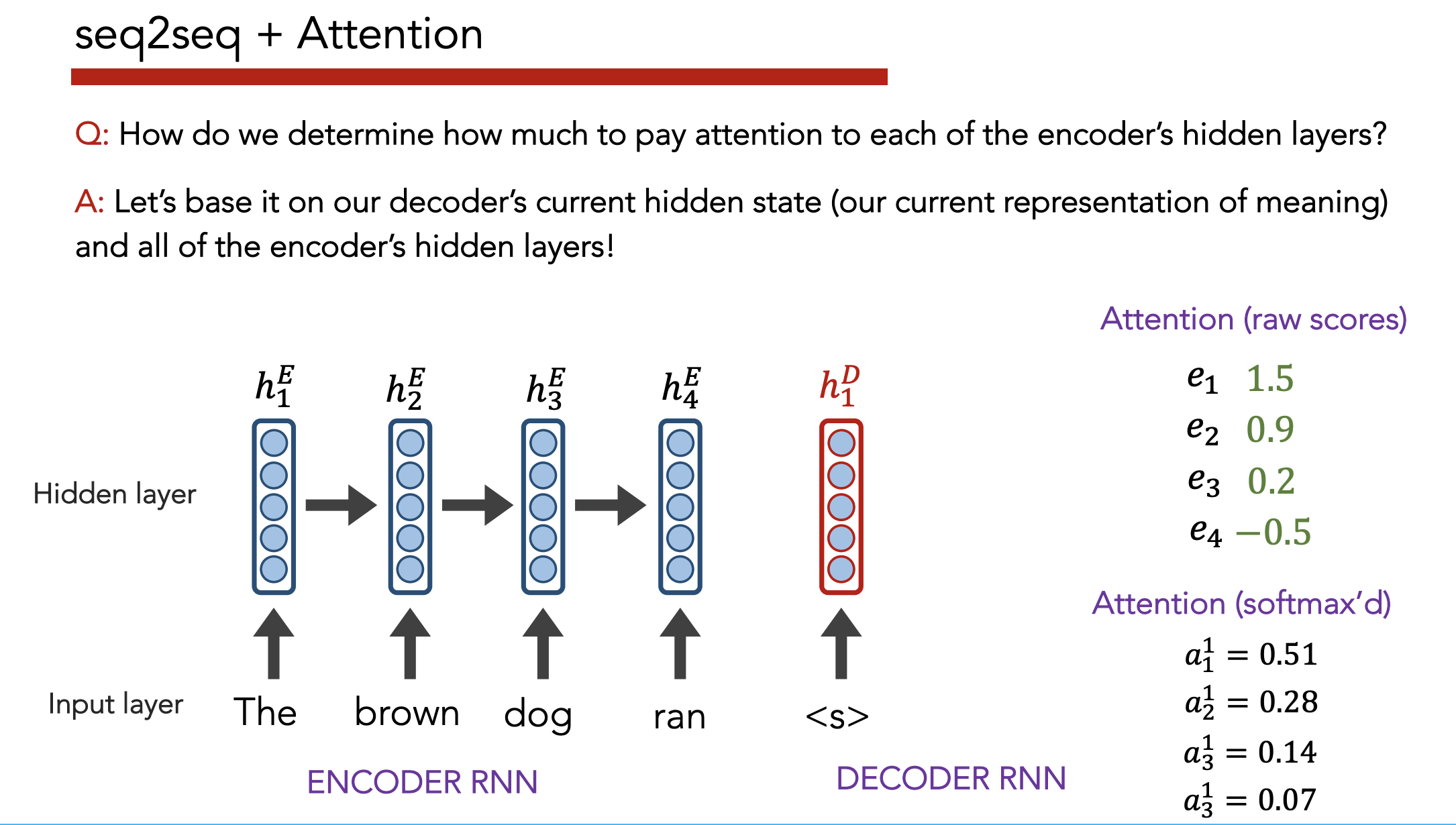
- Multiply each hidden state $h_i^E$ by $a_i$, then sum across all hidden states to get a context vector $c_j^D$
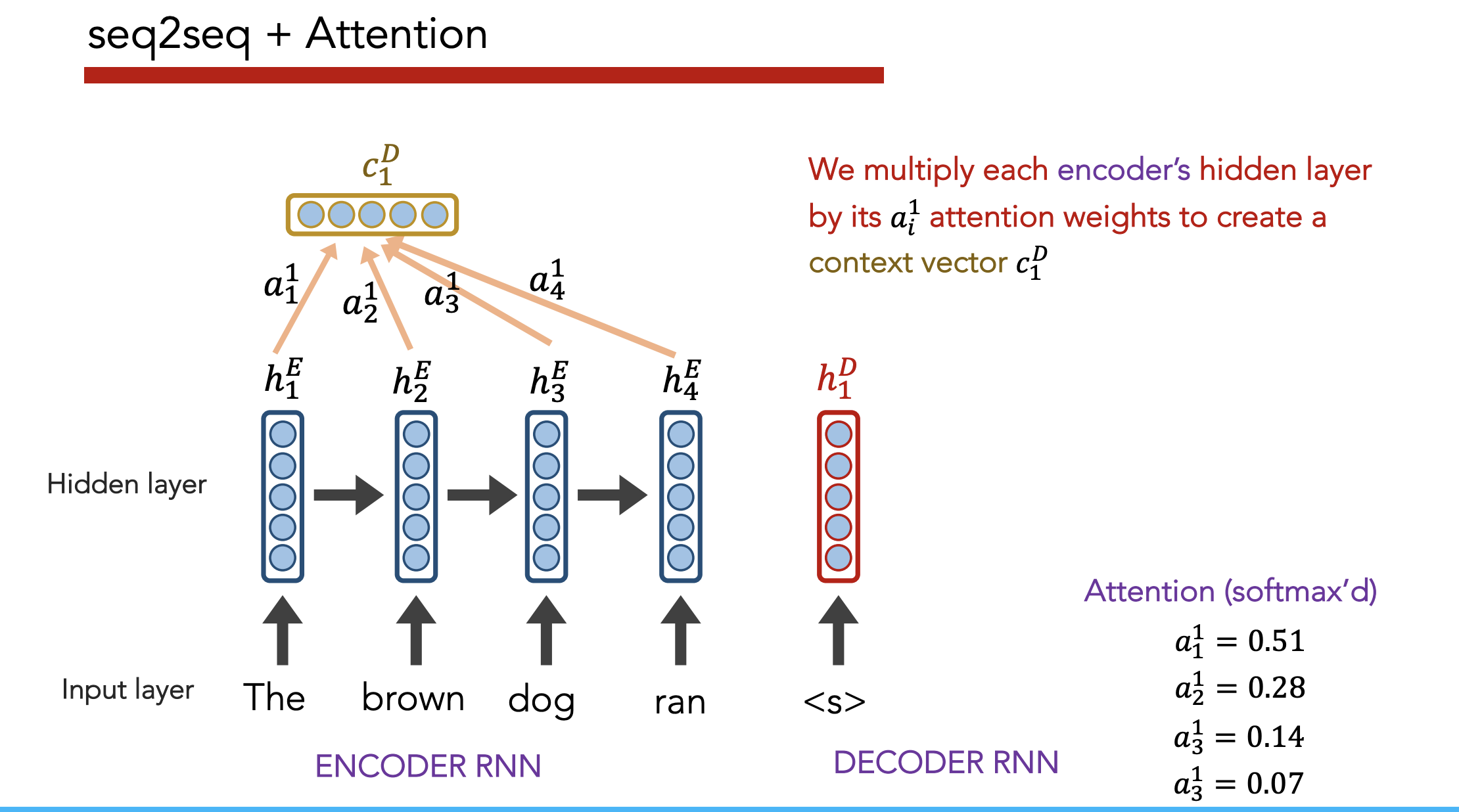
- Use $h_j^D, c_j^D$ to predict $\hat{y}_j$
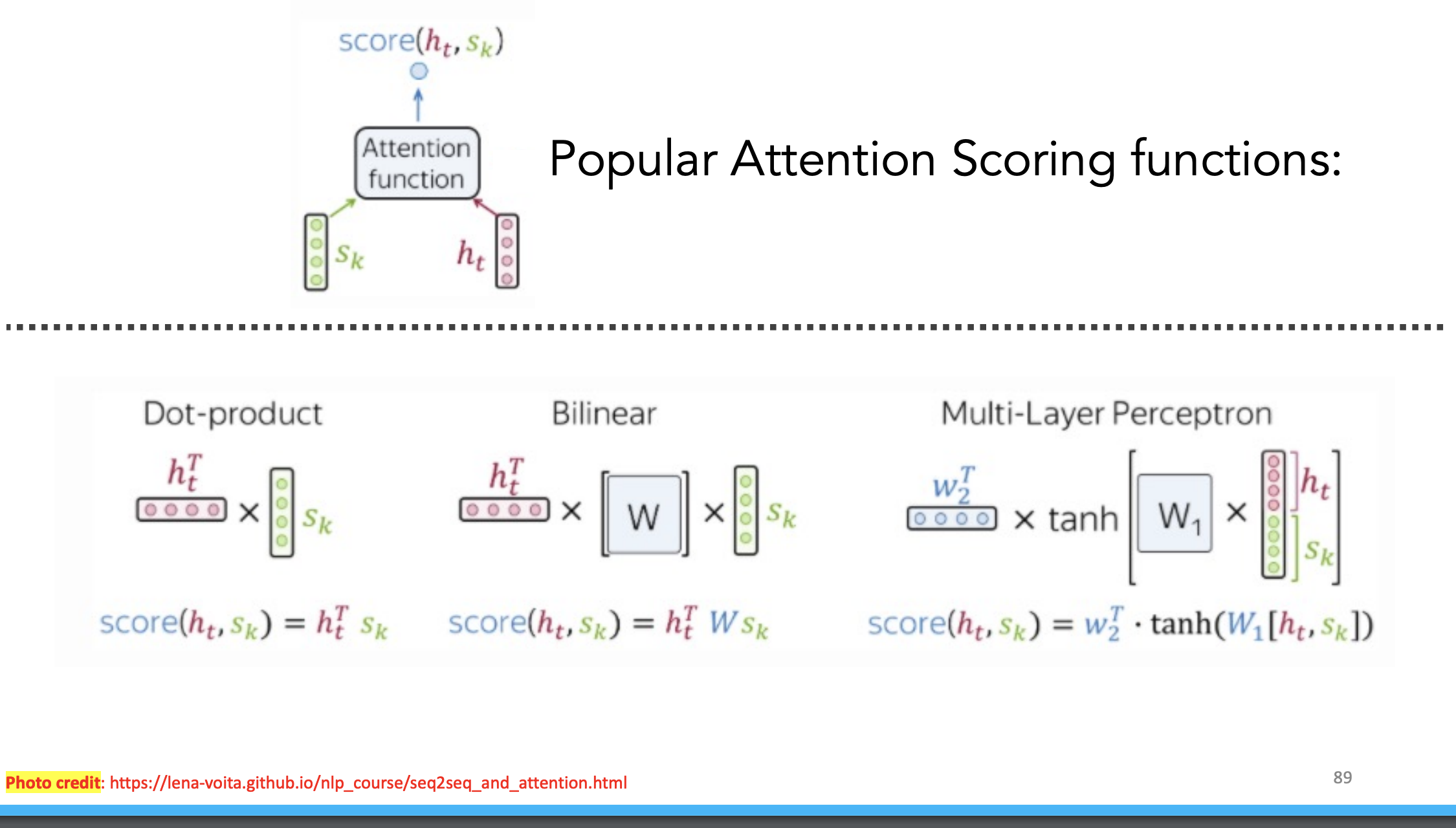
Attention Formulas + Functions
Benefits
- Greatly improves seq2seq results by conditionally weighting model’s focus
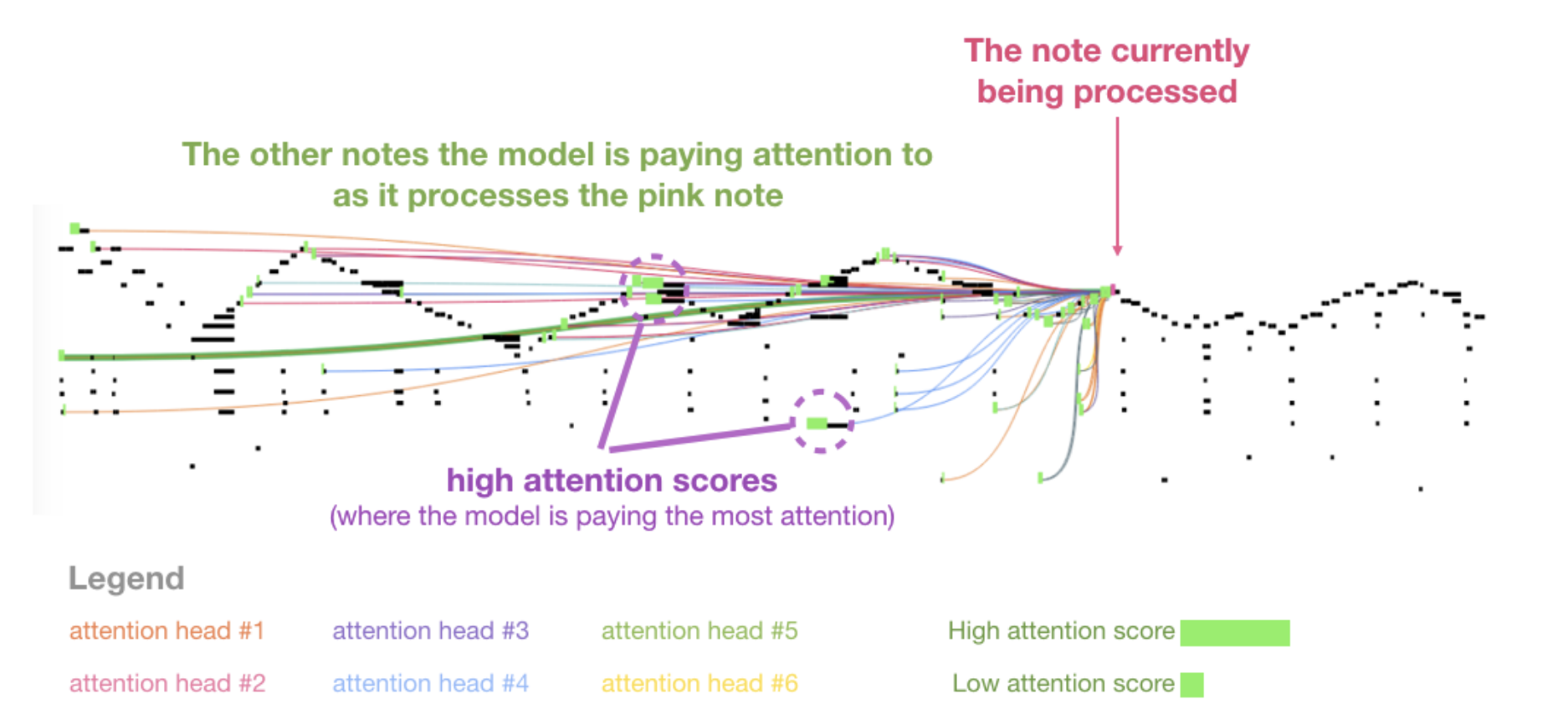
- Allows us to visualize contribution that each encoding word has for each decoder output
Summary
- LSTMs was SoTA on most NLP (2014-18)
- Seq2seq + Attention is even better
- Place appropriate weight on encoder’s hidden states when decoding
- Drawback: LSTMs still require iteratively reading each word and waiting until we’ve read the entire sentence before we can start predicting
8) Machine Translation [Source]
**Definition: ** Machine translation (MT) = convert text from one language into another
Seq2Seq Decoding for MT
Greedy Decoding: Pick most likely word at each step
Beam Search: Sequentially consider $k$ most likely words at each step. Prune before expanding
__TODO: Add here__
Strengths / Issues of Seq2Seq
Strengths:
- SoTA performance
- Uses context robustly
- Minimal feature engineering
- End-to-end optimization
Issues:
- OOV
- Training data (domain mismatch, low resource languages, biases)
- Long context still hard
- Not interpretable
- Hard to control
- Exploding/vanishing gradient issues
BLEU Score
“Bilingual Evaluation Understudy”
Purpose:
- Eval metric that measures similarity between gold-standard and candidate translation
Interpretation:
- Perfect match: $s = 1$
- Perfect mismatch: $s = 0$
The BLEU metric ranges from 0 to 1. Few translations will attain a score of 1 unless they are identical to a reference translation. For this reason, even a human translator will not necessarily score 1. […] on a test corpus of about 500 sentences (40 general news stories), a human translator scored 0.3468 against four references and scored 0.2571 against two references.
Approach:
- Weighted geometric mean of “modified n-gram precisions” for $n \in {1, 2, 3, N }$, multipled by a “brevity penalty” for translations that are too short
- Typically use $N = 4$, i.e. use 4-gram as maximum n-gram size
- “Clip” repeated n-grams, i.e. treat sentence as a set of n-grams where repeated words count only once
“The primary programming task for a BLEU implementor is to compare n-grams of the candidate with the n-grams of the reference translation and count the number of matches. These matches are position-independent. The more the matches, the better the candidate translation is.”
Unigram Precision = % of unigrams in the model’s output sentence that occur in at least one reference translation
Formula [Source]
Let…
- $\hat{y}^x$ be the candidate translation for $y^{(i, x)}. \forall i \in S$
- $\hat{S}$ be the set of candidate translations
-
Let $ \hat{S} = M$ be the number of candidate translations
-
- $S$ be the set of reference translations for each candidate translation
-
Let $ S_i = N_i$ be the number of reference translations for translation $i$ - e.g. for $\hat{y}^x \in \hat{S}$, there is a set of reference translations $y^{(x, 1)}, …, y^{(x, N_i)} \in S_i$ taken from $N_i$ different reference sources
-
- $w_n$ be the weight assigned to the $n$-grams
- $W$ be max $n$-gram length
- $r$ be the length of the reference corpus
- $c$ be the length of the candidate corpus
Where… \(C(s, y) = \text{\# of times $s$ appears as substring of $y$}\\ G_n(y) = \text{set of $n$-grams in $y$}\\ \sum_{s \in G_n(\hat{y})} C(s, y) = \text{\# of total occurrences that $n$-grams in $y$ appear in $\hat{y}$}\)
Example [Source]
Let…
-
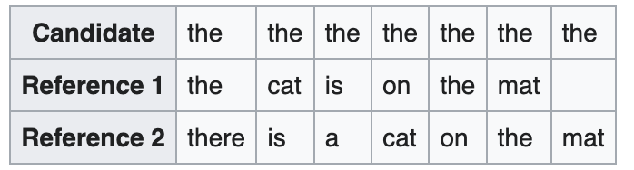
$m$ = # of words in candidate that are found in the reference set
-
$w_t$ = total # of words in candidate
Unigram Precision $P$: \(P = \frac{m}{w_t} = \frac{7}{7} = 1\)
Let…
- $m_{max}$ = max total count of a word in any of the reference translations
Modified Unigram Precision $P$:
\(P = \frac{m_{max}}{w_t} = \frac{2}{7}\)
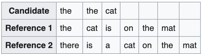 \(\begin{align*}
\text{Unigram Precision} &= \text{"the", "the", "cat"} = \frac{1 + 1 + 1}{3} = 1\\
\text{Modified Unigram Precision} &= \text{"the", "cat"} = \frac{1 + 1}{3} = \frac{2}{3}\\
\text{Bigram Precision} &= \text{"the the", "the cat"} = \frac{0 + 1}{2} = \frac{1}{2}\\
\text{BLEU} &= \text{weighted geometric mean of above entries}
\end{align*}\)
\(\begin{align*}
\text{Unigram Precision} &= \text{"the", "the", "cat"} = \frac{1 + 1 + 1}{3} = 1\\
\text{Modified Unigram Precision} &= \text{"the", "cat"} = \frac{1 + 1}{3} = \frac{2}{3}\\
\text{Bigram Precision} &= \text{"the the", "the cat"} = \frac{0 + 1}{2} = \frac{1}{2}\\
\text{BLEU} &= \text{weighted geometric mean of above entries}
\end{align*}\)
Strengths / Issues of BLEU [Source]
Pros:
- Fast and simple
Cons:
- Ignores meaning
- Ignores sentence structure
- Assumes sentence is already tokenized (so must use same tokenizer to compare different models)
- Solution: Use
SacreBLEUas alternative method
- Solution: Use
9) Self-Attention
Issues with LSTMs:
- Unparallelizable (sequential in nature)
- No explicit modeling of long- and short-range dependencies
- We don’t use attention to craft our encoder representations
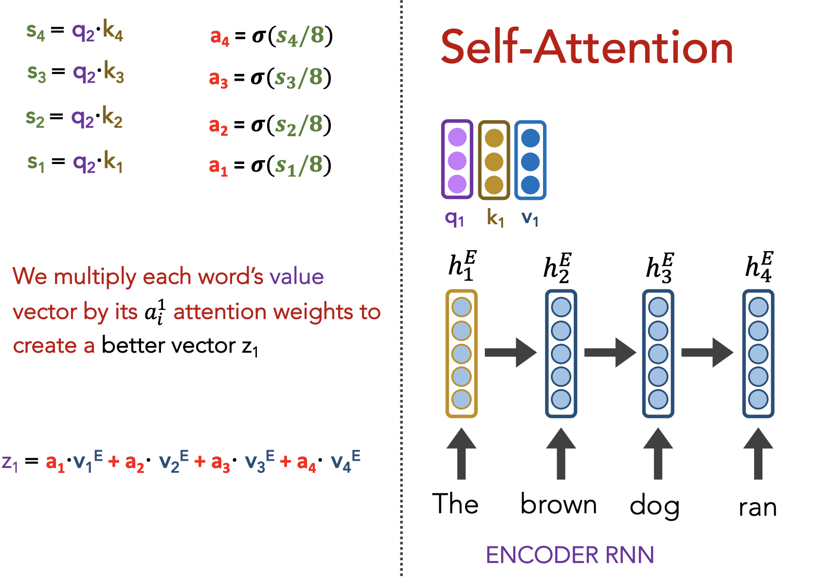
Question: Can we use attention to improve not just our decoder’s output, but also our encoder’s contexutalized representations (i.e. embeddings)?
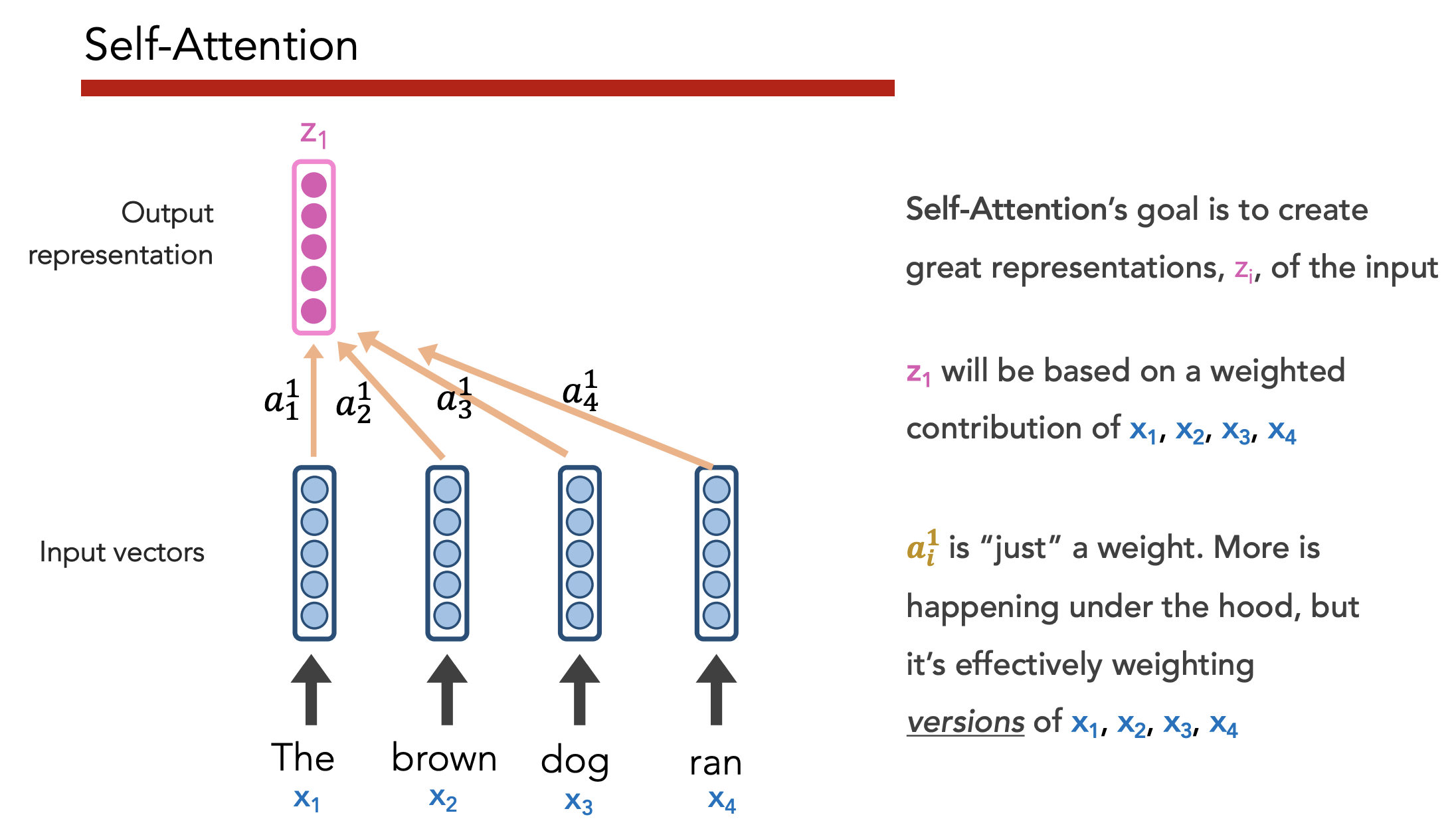
Goal:
- Have each word determine how much it should be influenced by its neighbors
- Preserve positionality
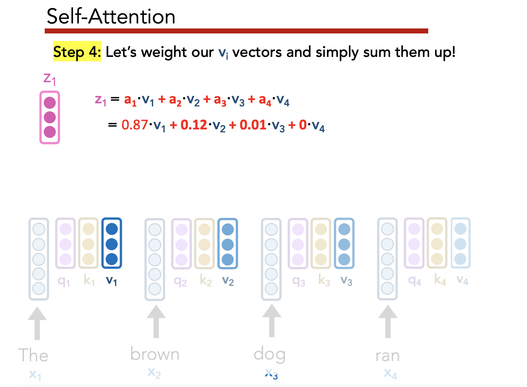
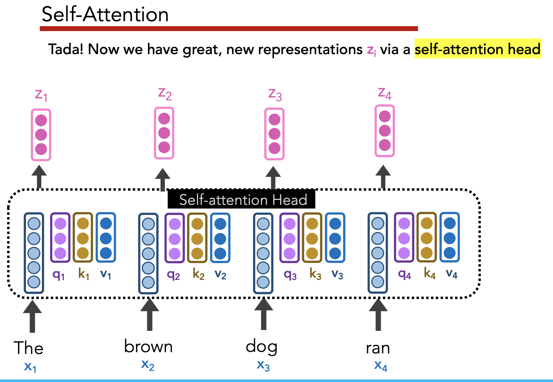
Self-attention allows us to “create great, context-aware representations”
10) Transformers
Self-Attention v. Seq2Seq Attention
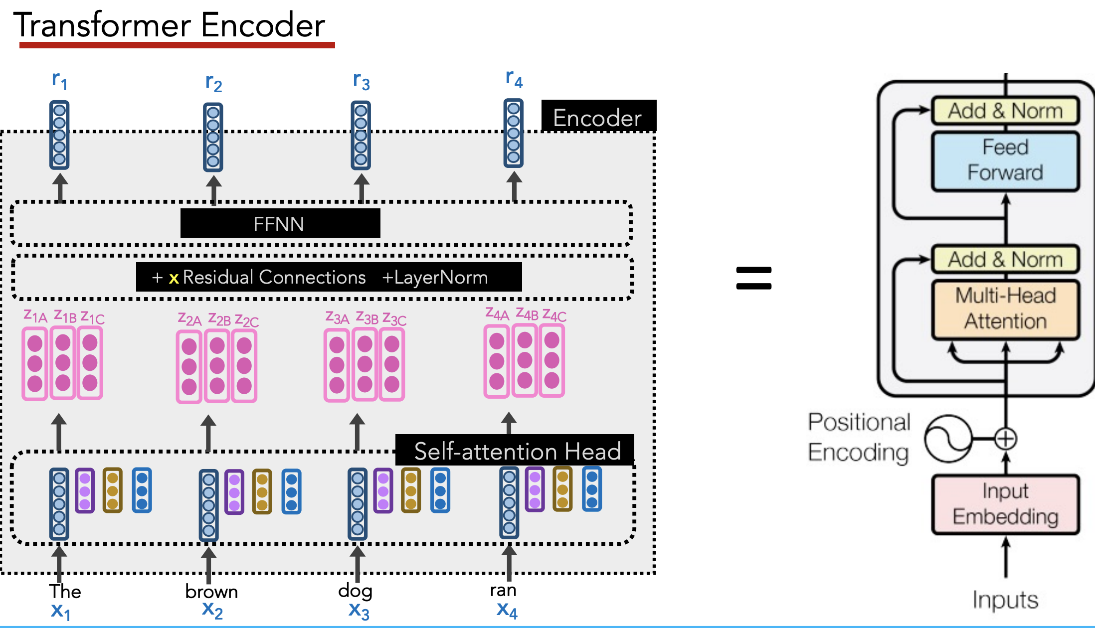
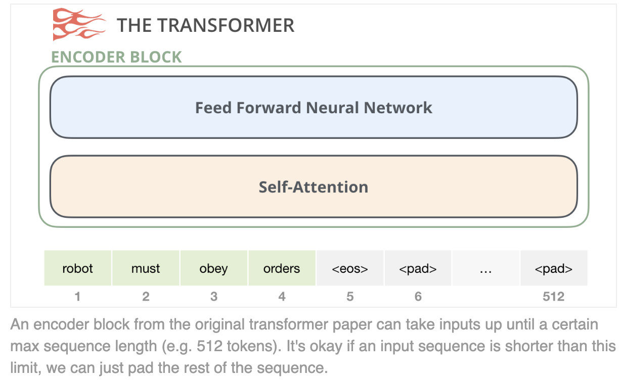
Transformer Encoder
Goal: Create good contextualized embedding $r_i$ for each word $x_i$
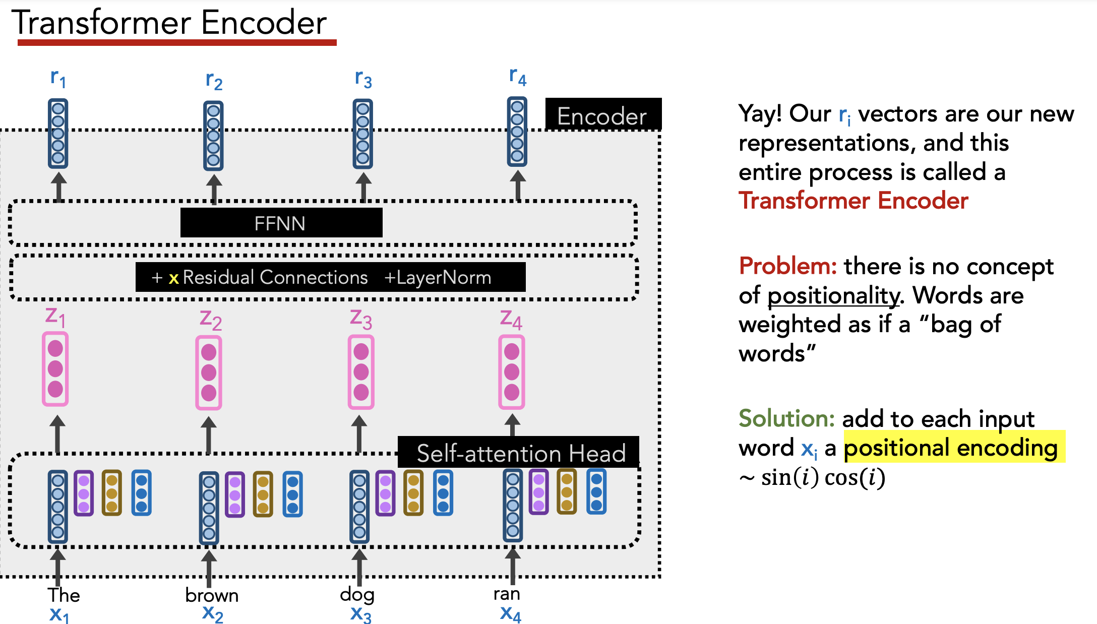
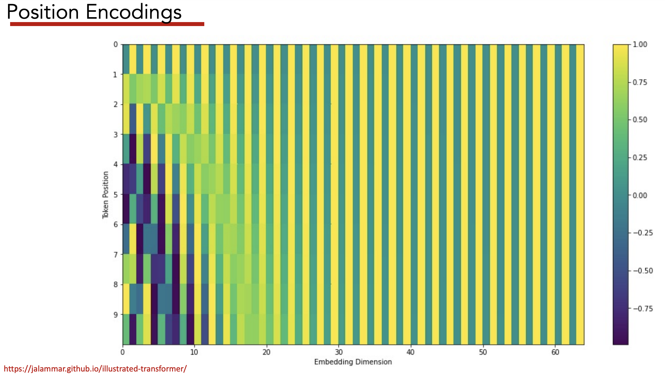
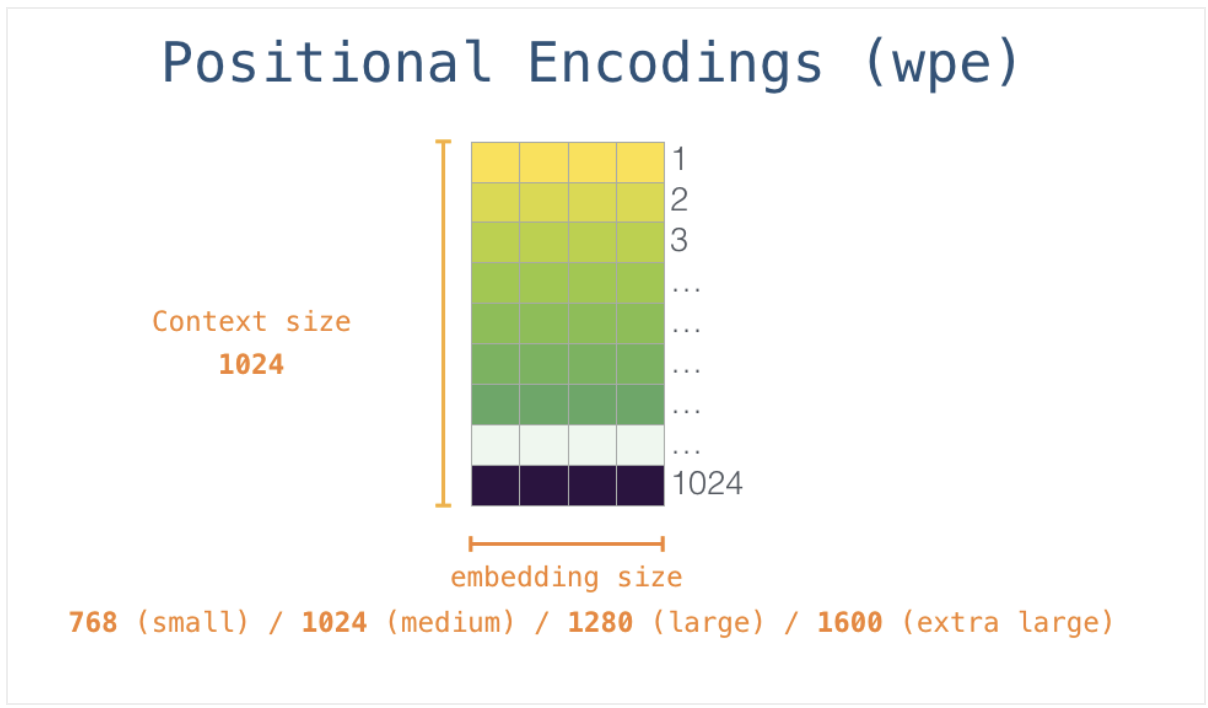
Position Encodings
Under the set-up above, ordering of words is ignored by model.
Need to add positional info to each word’s embedding to preserve positional info.
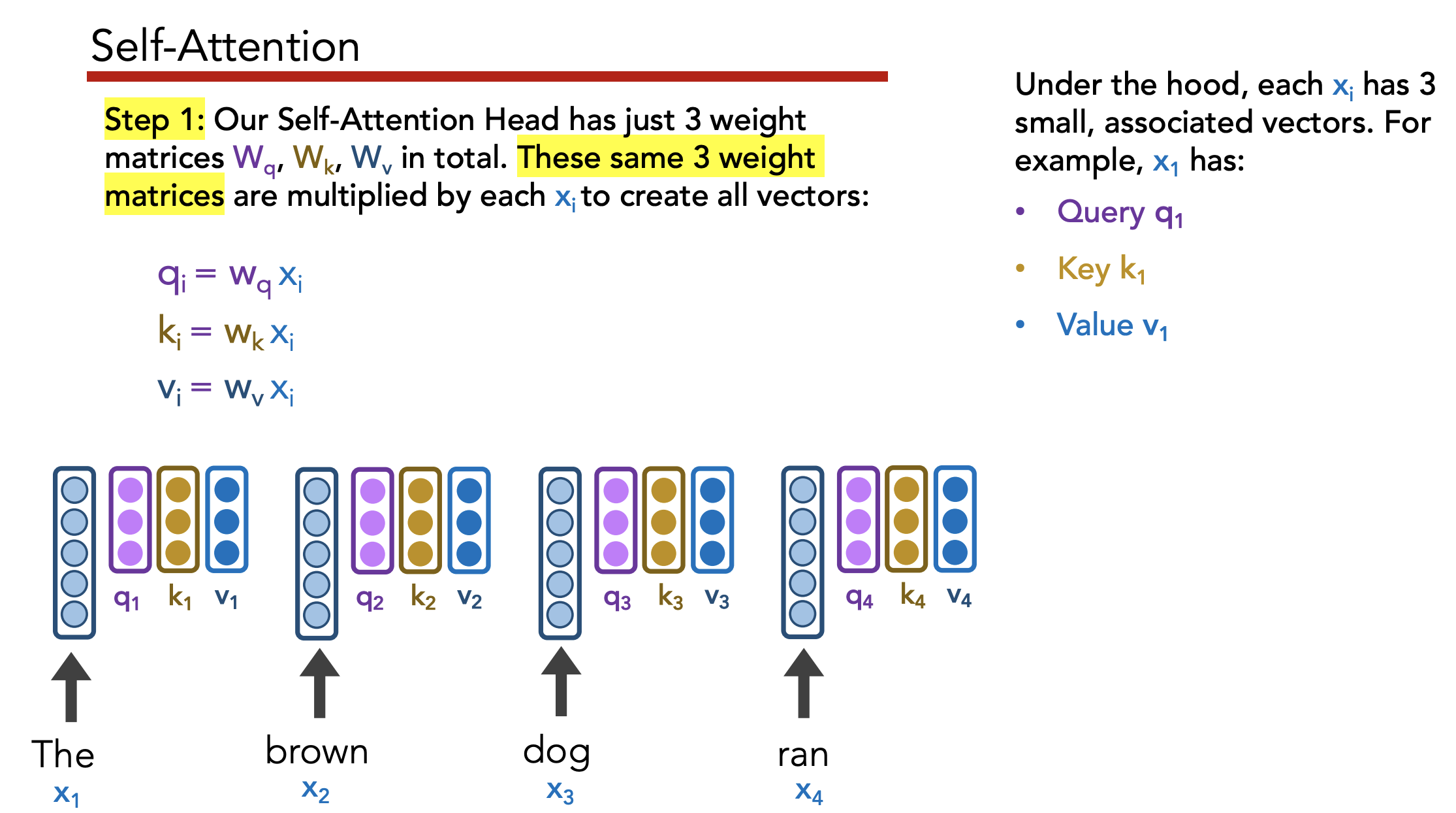
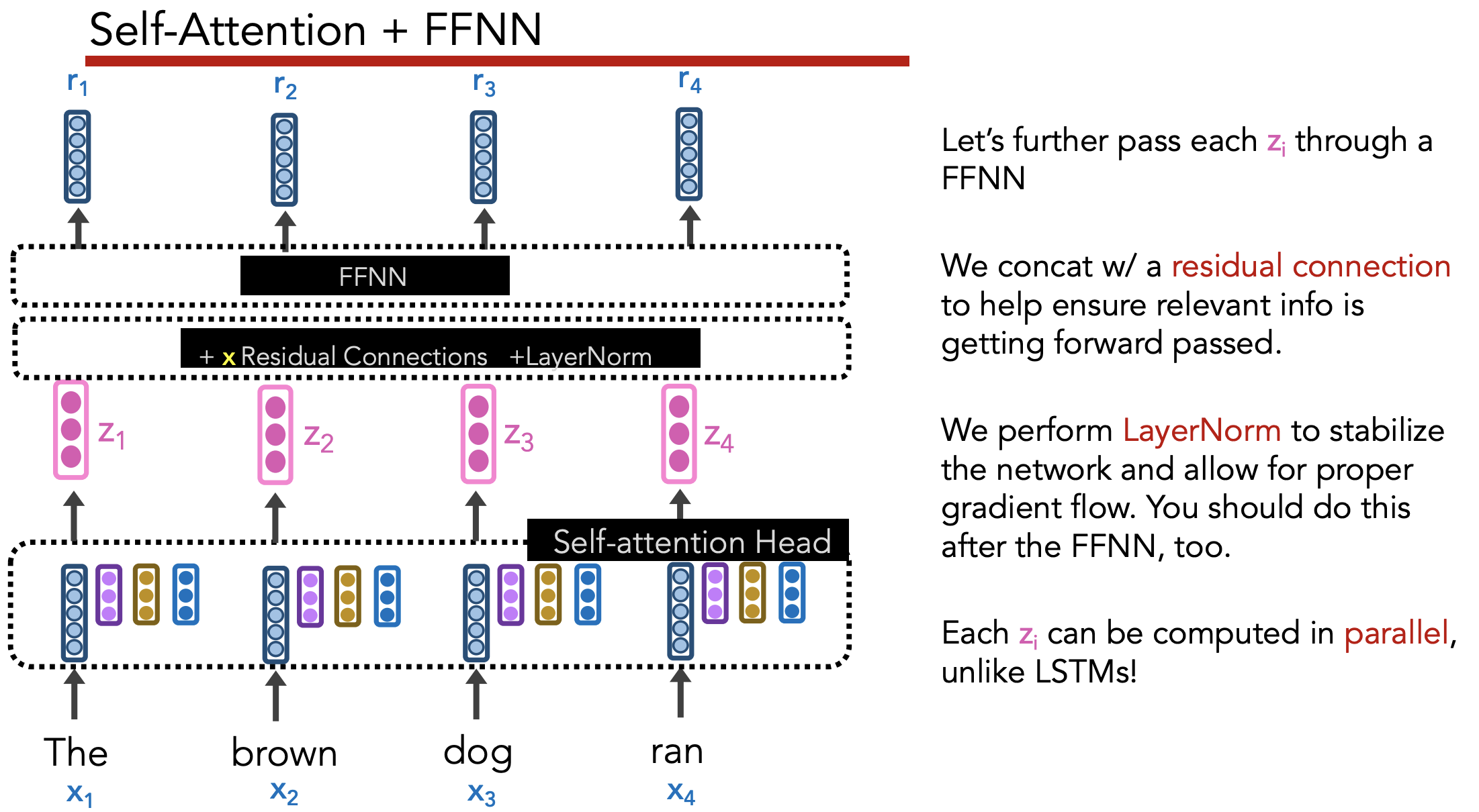
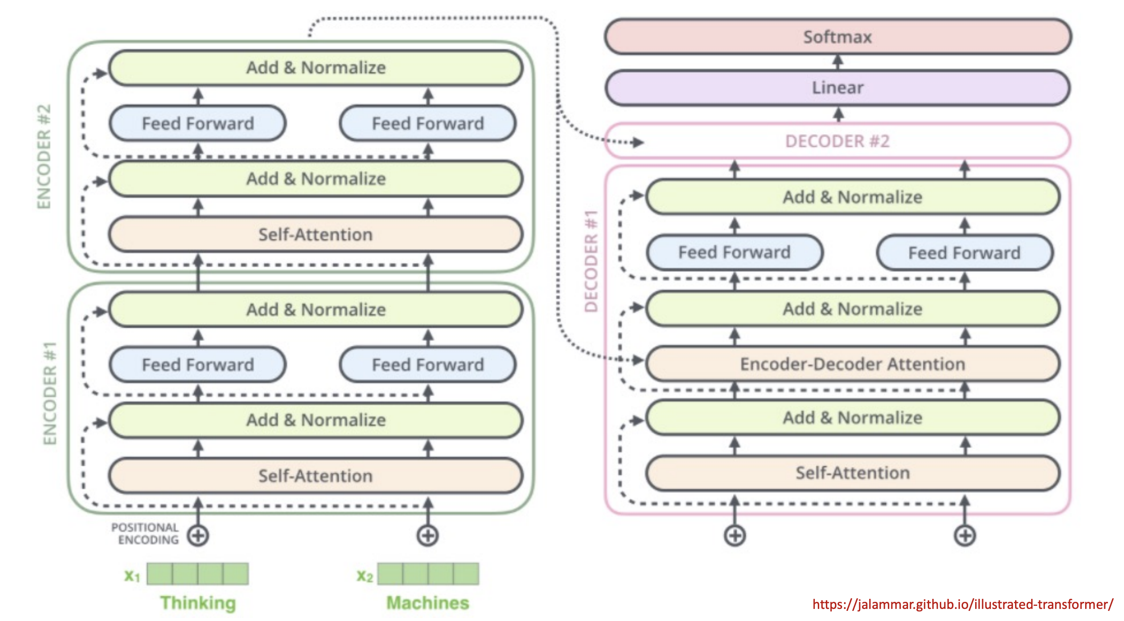
Multi-head attention: Have multiple query/key/value matrices $W_q, W_k, W_v$, then concatenate the $z_i$’s they generate.
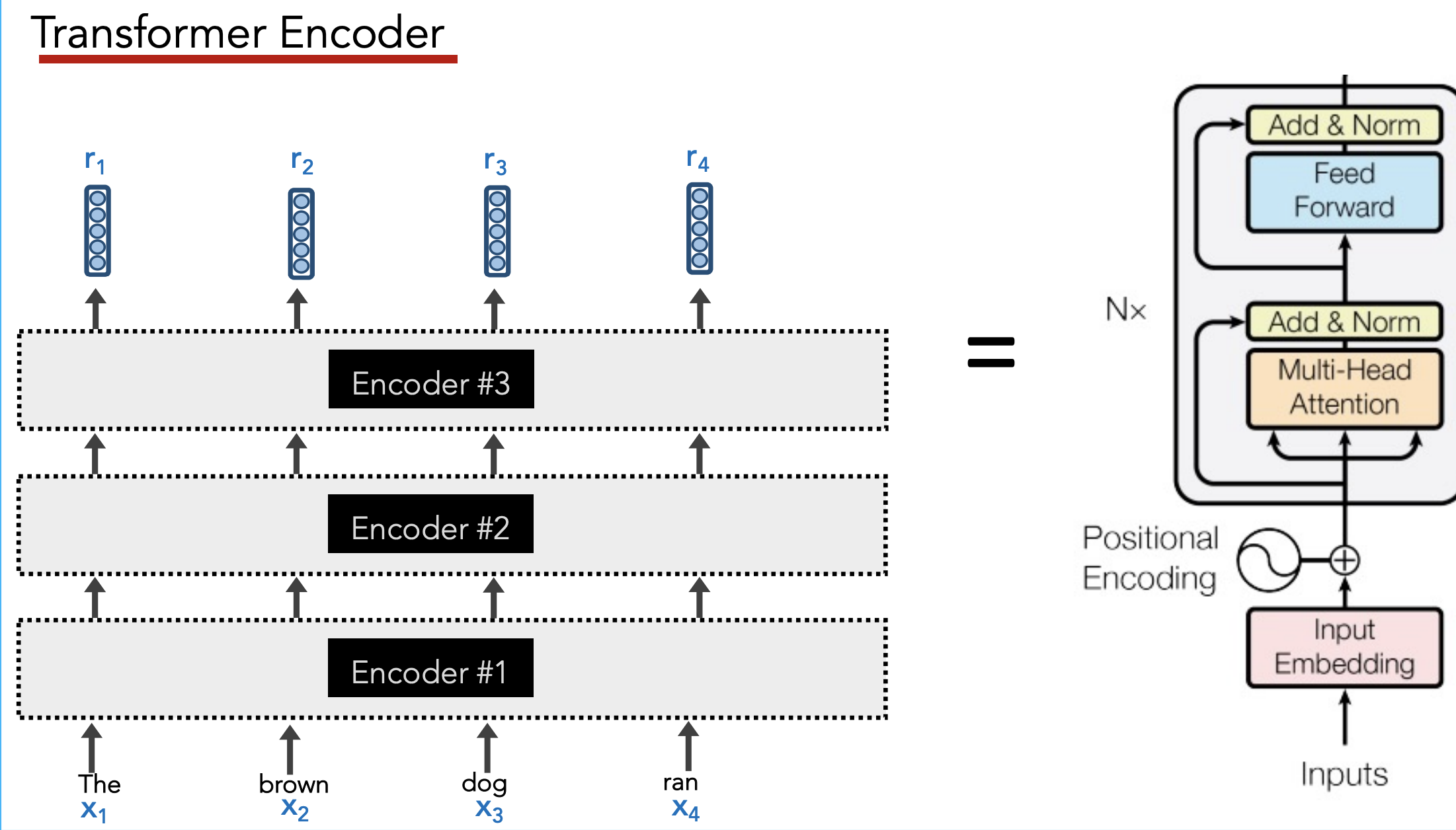
Stack multiple transfomers together:
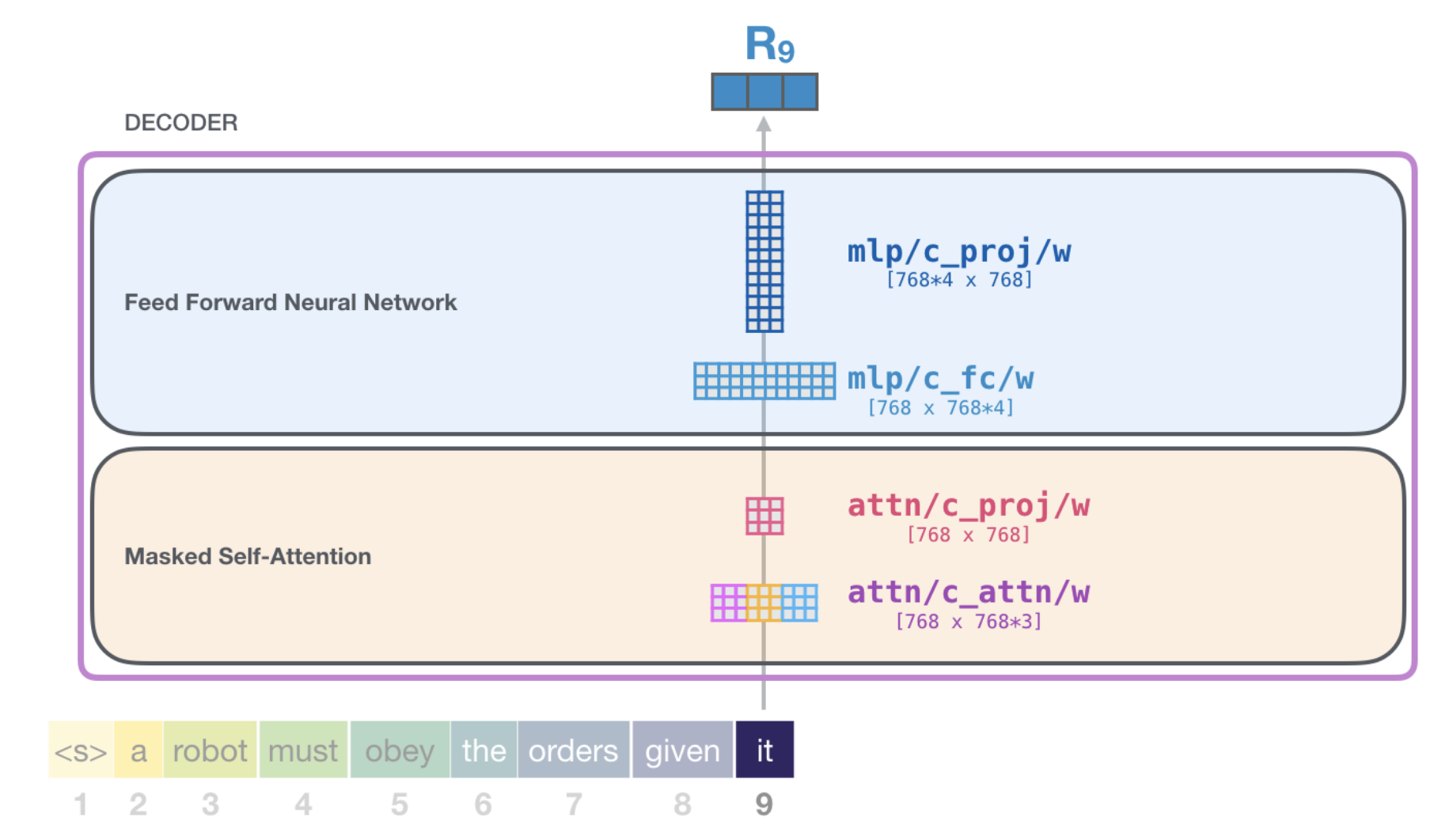
Transformer Decoder
Goal: Generate new sequence of text
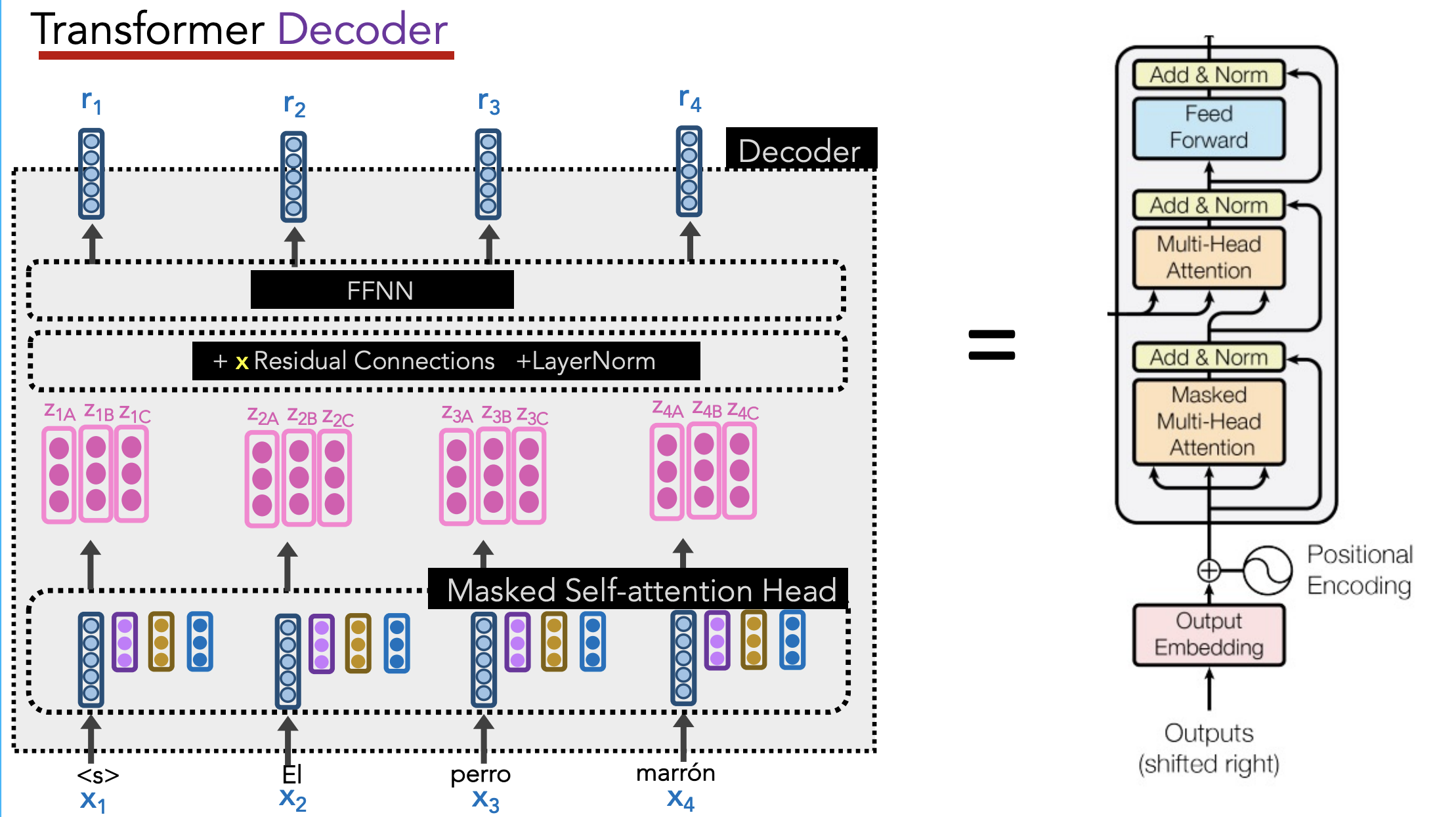
Decoder has two attention heads:
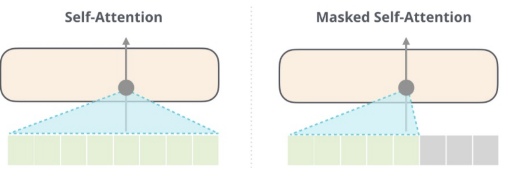
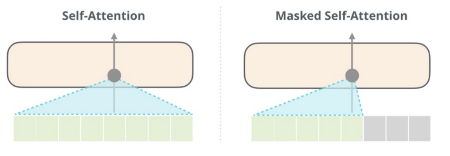
- Masked Multi-Head Attention (aka “Self-Attention Head”)
- query, key, value = outputs of the previous decoder layer
- Each position can only attend to previous words (so mask future words) – preserves auto-regressive LM behavior
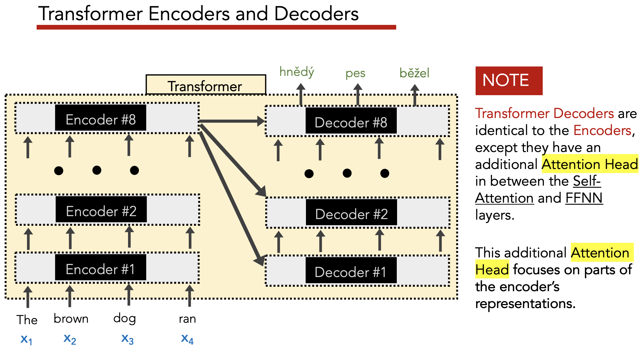
- Multi-Head Attention (aka “Attention Head”) in between the Self-Attention and FFNN layers
- query = output of the previous decoder layer
- key, value = outputs of the encoder
Overview Diagrams
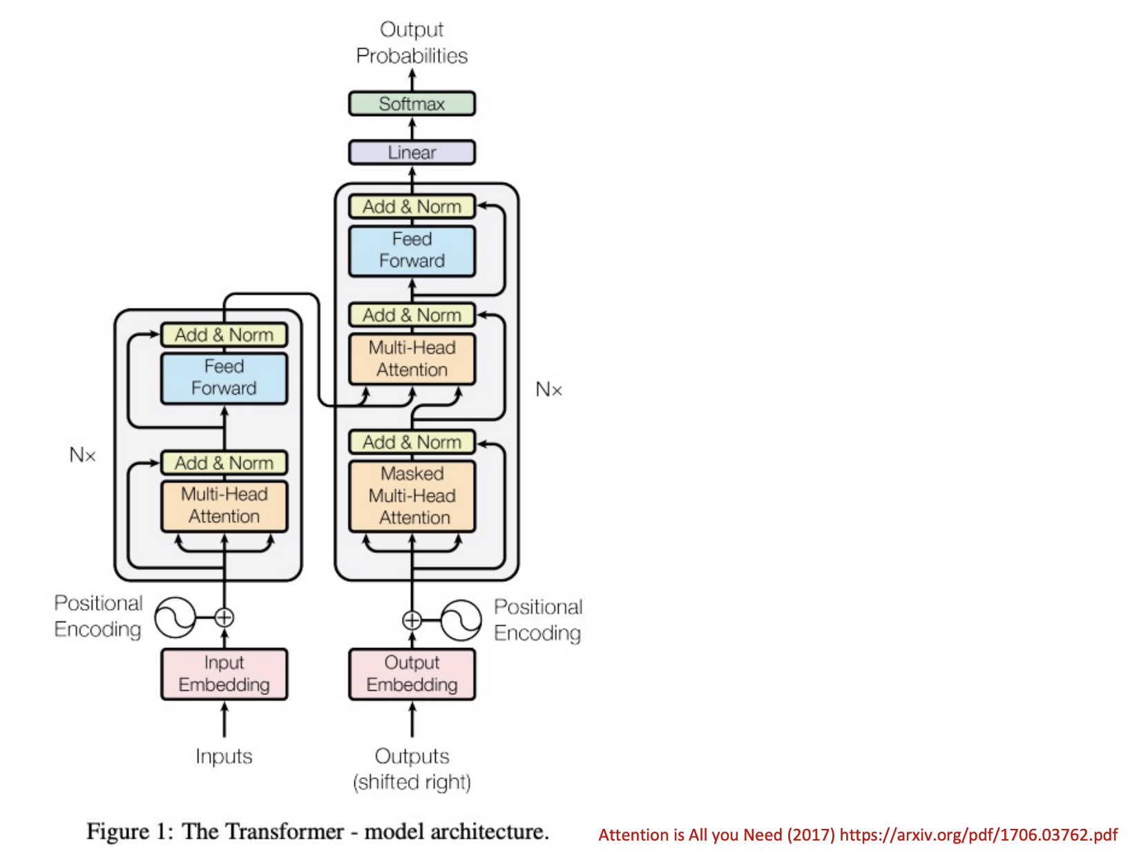
Loss function: Cross-entropy of output word
Simplified Encoder Diagram
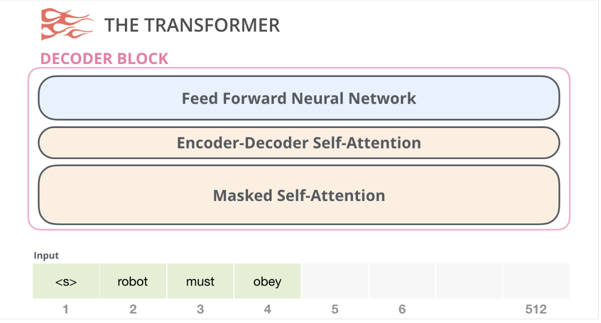
Simplified Decoder Diagram
Two key differences from Encoder:
- Has attention over Encoder’s outputs
- Has masked self-attention which masks out future tokens
Types of Attention
- Encoder-Decoder Attention: Decoder attends to all of encoder’s inputs
- Encoder Self-Attention: Encoder attends to all of its inputs
- Decoder Masked Self-Attention: Decoder attends to all of its prior outputs
BERT uses encoder self-attention
GPT-2 only uses decoder masked self-attention
Big-O Analysis
Let…
- $n$ = input sequence length
- $d$ = length of embedding vector
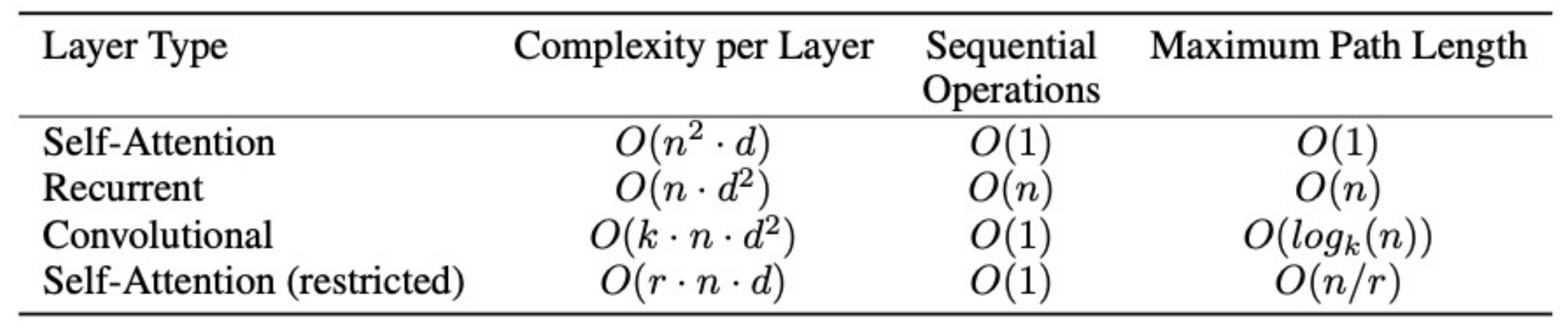
Shorter maximum path lengths = stronger learned dependencies between words
11) BERT
Model Categorization
Types of Data
Unlabeled
- Raw text (web pages, books)
- Parallel corpora (translations)
Labeled
- Unstructured
- N-to-1 (sentiment analysis)
- N-to-N (POS tagging)
- N-to-M (summarization)
- Structured
- Dependency parse trees
- Constituency parse trees
- Semantic role labelling
Types of Learning
Style of Learning
- Multi-task: Train on multiple tasks
- Transfer learning: Subset of multi-task learning where we only care about one downstream task
- Pre-training: Subset of transfer learning where we first focus on one task, then apply it to multiple downstream tasks
Ideally, tasks are closely related
Multi-task is most useful on tasks with limited data.
Type of Data Available
- Supervised
- Unsupervised
- Self-supervised
- Semi-supervised
BERT (Bidirectional Encoder Representations from Transformers)
Goal: Language model that builds rich representations
Structure
Model: Transformer encoders (xN)
Data:
- Input a “sequence”, which is simply a list of tokens that can represent either 1 or 2 sentences
<SEP>to separate sentences within a sequence- Also add a learned embedding to each token to indicate if its in the 1st or 2nd sentence
<CLS>is always the 1st token of each sequence, and rerpesents aggregate sequence representation- Use WordPiece embeddings with a 30k token vocab
Objectives:
- Masked language modeling (“MLM”), i.e. predict masked word
- Next-sentence prediction (“NSP”), i.e. predict if two sentences are next to each other
Data:
- BooksCorpus
- Wikipedia
Training Objectives
-
Predict a masked word (e.g. CBOW)
- 15% of input words randomly masked
- 80% =>
[MASK] - 10% => revert back
- 10% => deliberately wrong words
- 80% =>
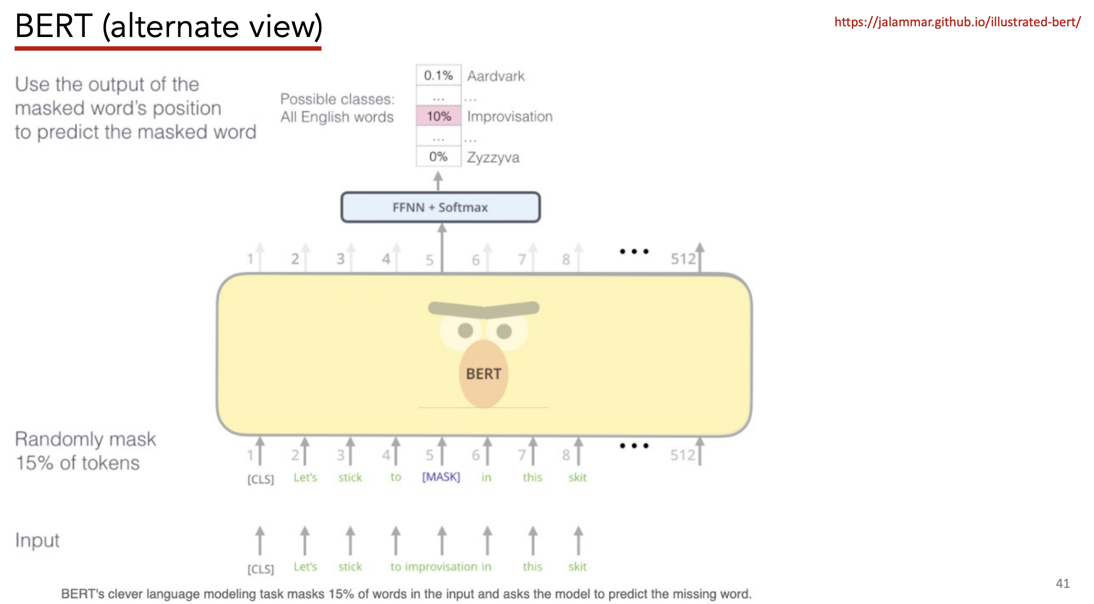
- 15% of input words randomly masked
-
Given two sentences, predict if the second follows the first
- Start the first sentence with a
<CLS>token - Separate each sentence with
<SEP>token -
50% of the time, 2nd sentence actually follows 1s sentence 50% of time, 2nd sentence is randomly sampled from corpus - Make prediction based on embedding of
<CLS>token
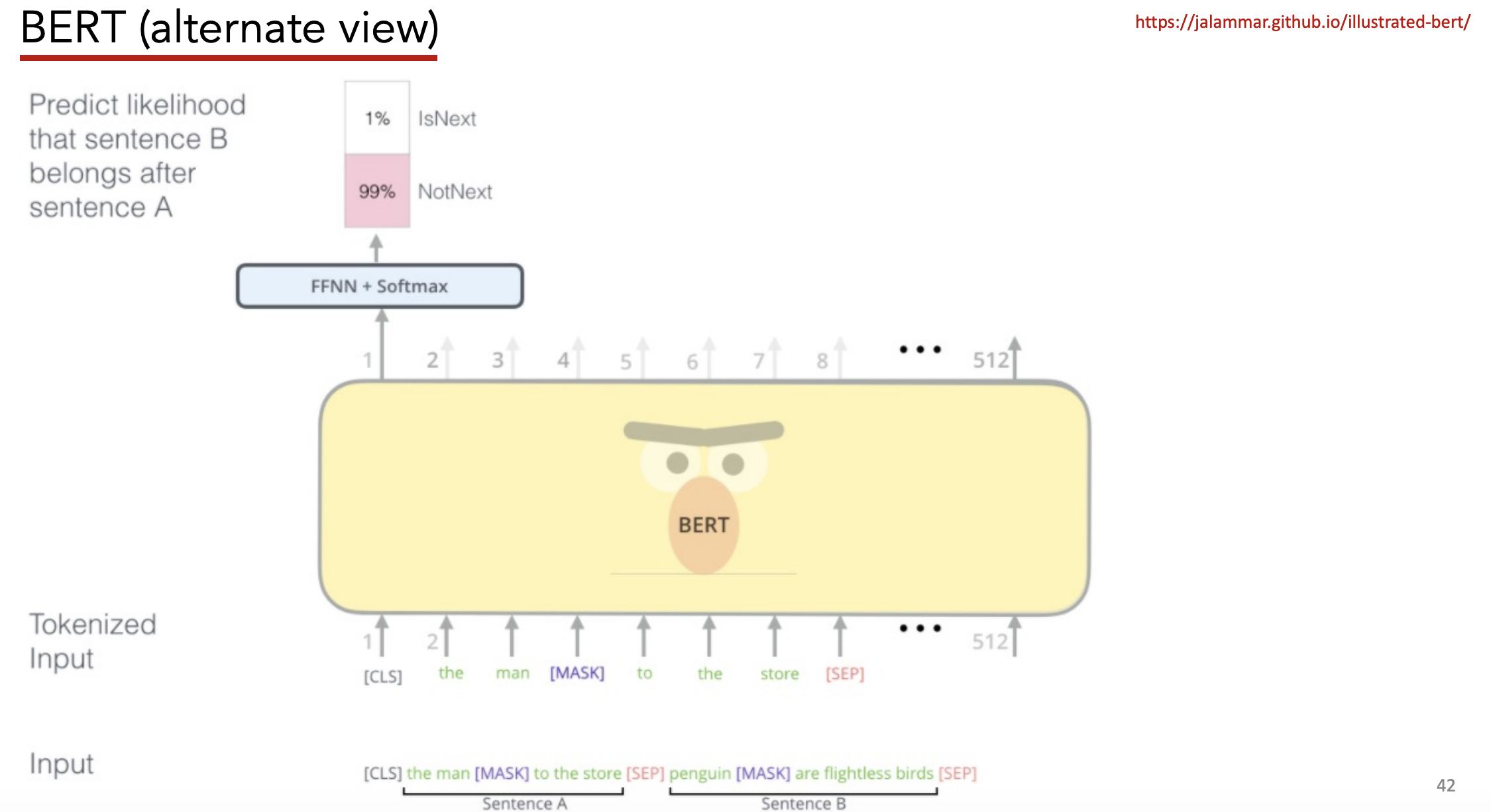
- Start the first sentence with a
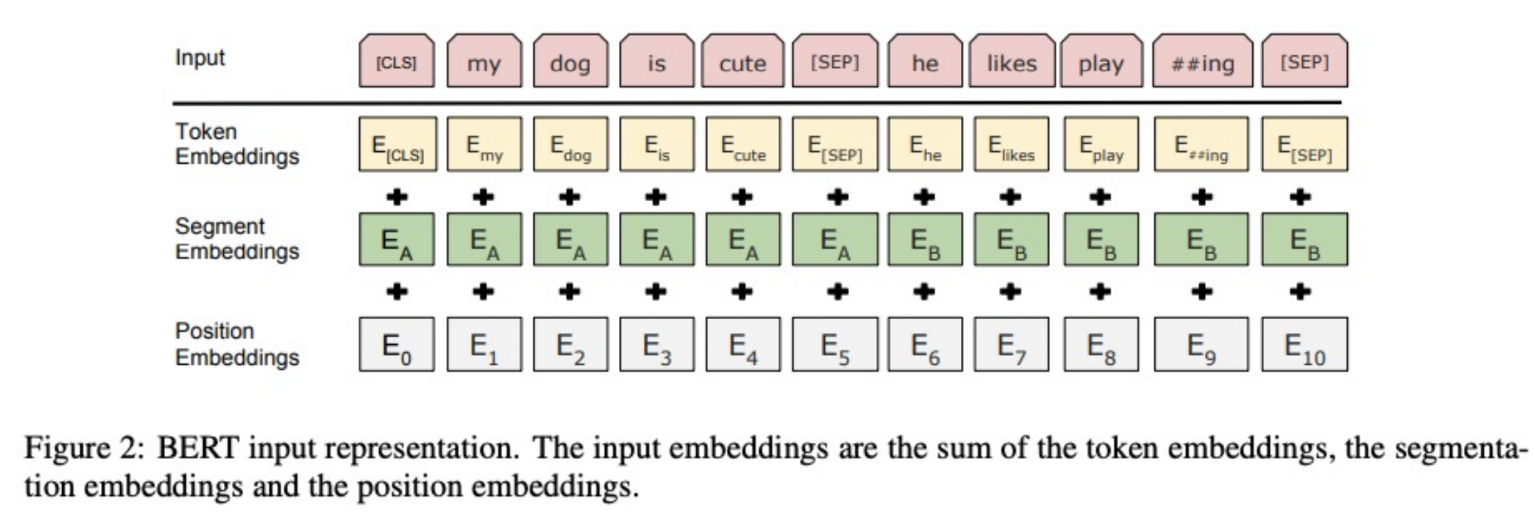
Inputs
Input tokens are represented as the sum of three embeddings:
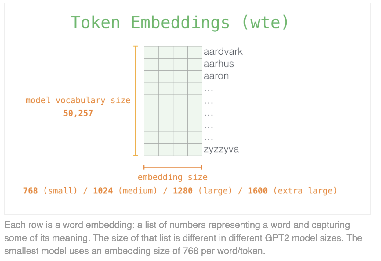
- Token embeddings – Taken from WordPiece, which is a “sub-word tokenization learns to merge and use characters based on which pairs maximize the likelihood of the training data if added to the vocab”
- Segment Embeddings – Indicates if token is from the 1st or 2nd sentence
- Position Embeddings – Indicates token’s position in overall sequence
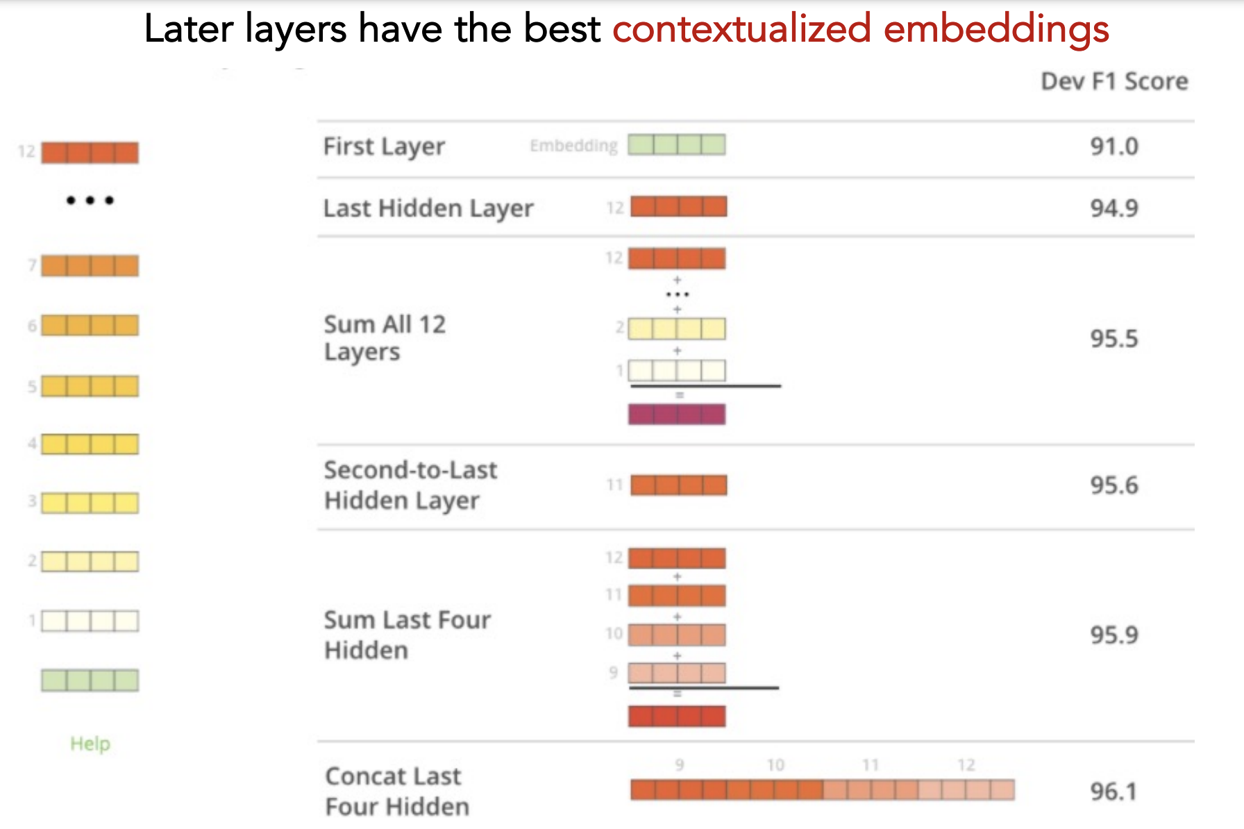
Outputs
Concatenate last 4 hidden layers to serve as contextualized embedding of input sentence
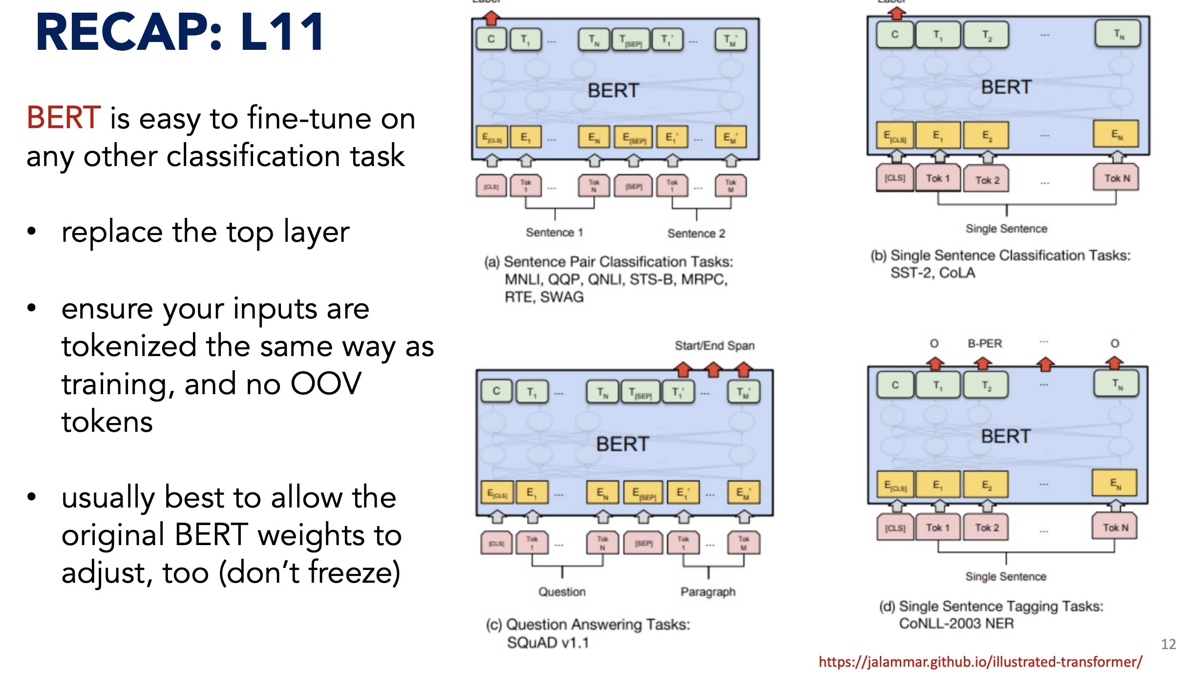
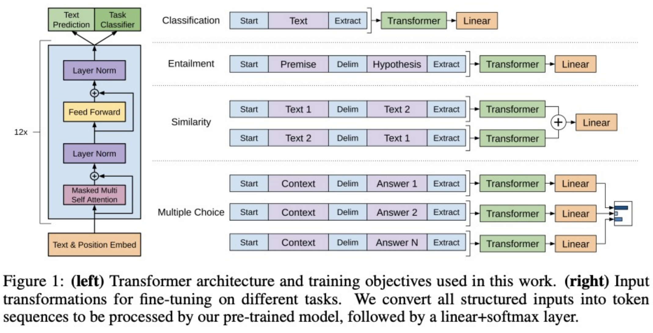
Fine-Tuning
Summary
Takeaway: BERT learns SoTA contextualized embeddings, great for downstream tasks (e.g. classification)
Limitation: Can’t generate new sentences b/c no decoder.
Extensions
Transformer-Encoders
- ALBERT - A Lite BERT
- RoBERTa - Robustly Optimized BERT
- DistilBERT - Small BERT
- ELECTRA - Pre-training Text Encoders as Discriminators not Generators
- Longformer - Long-Document Transformer
Autoregressive
- XLNet
- GPT - Generative Pre-Training
- CTRL - Conditional Transformer LM for Controllable Generation
- Reformer
12) GPT-2
Goal: Generate a new output sequence
Idea: Use only Decoders (no Encoders); use only self-attention ((no encoder-attention))
Differences with BERT
- BERT uses only encoders, GPT-2 only uses decoders
- BERT uses encoder-attention, GPT-2 only uses self-attention
- GPT2 is autogressive – BERT is not
- Autogression = use previous outputs as model inputs
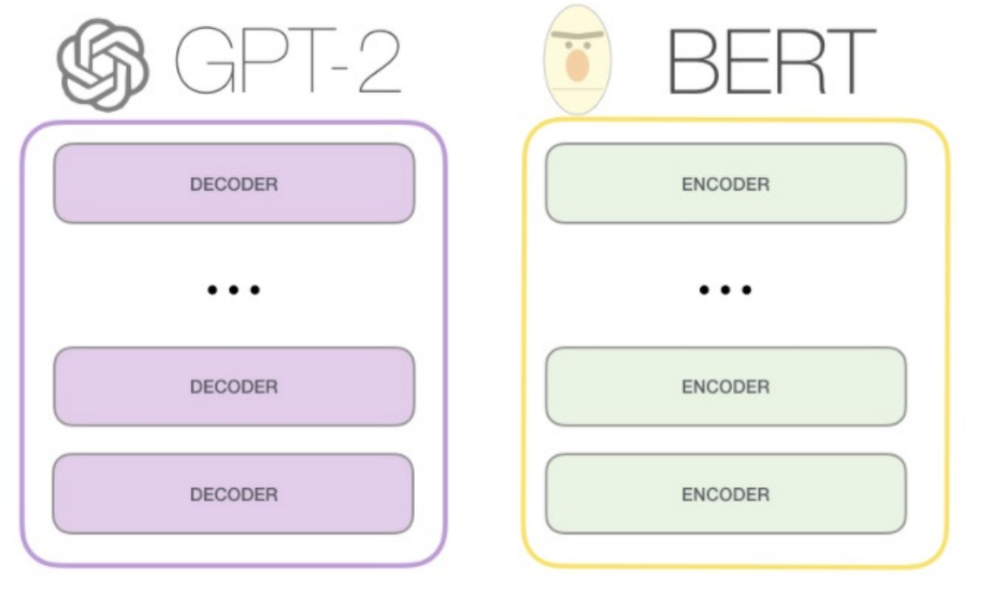
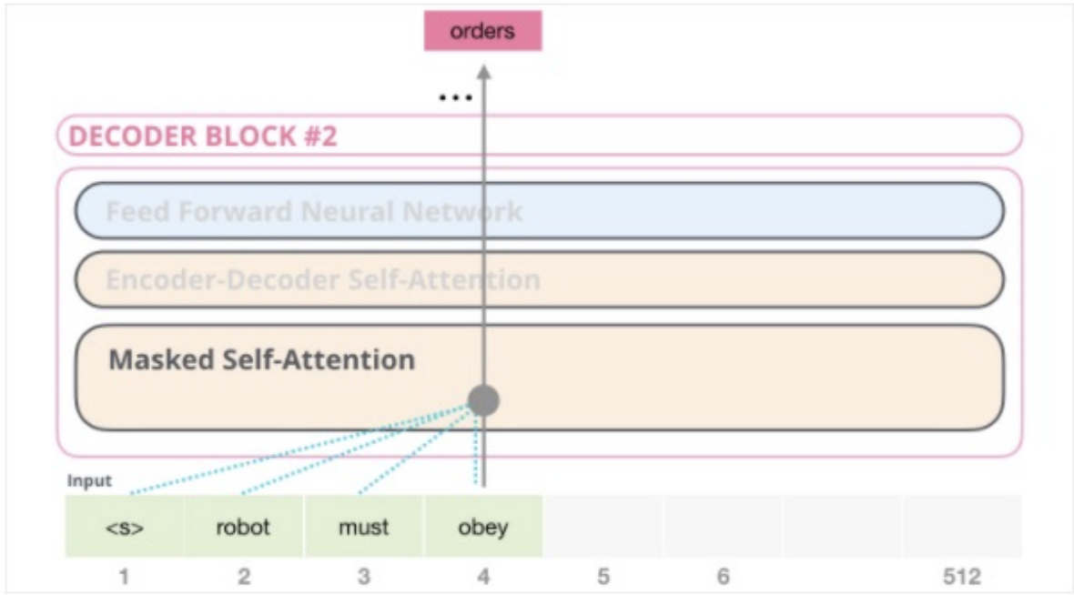
It only uses masked self-attention (mask out future words)
Input
- Uses BytePair Encodings (i.e. sub-words) instead of words, similar to BERT’s WordPieces
BytePair Encodings (BPE)
Look at individual characters and repeatedly merge most frequent pairs (e.g. agglomerative clustering)
Stops after $N$ merges. GPT uses $N = 40k$
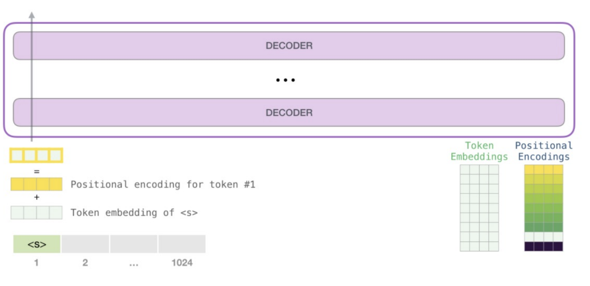
All 1,024 positions in the input are given a unique positional encoding
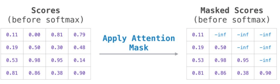
Masked Attention
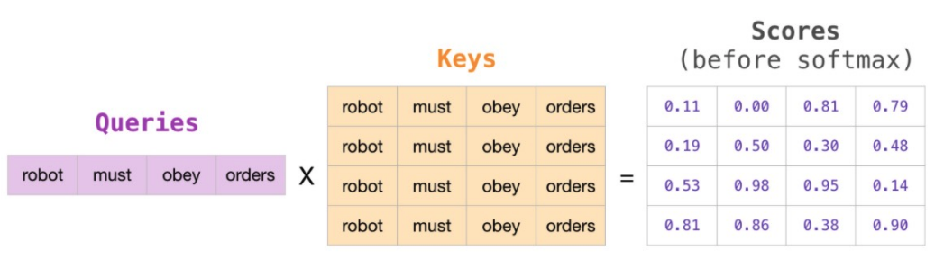
Top row of Scores is how much the word “robot” should attend to each of the other words (“robot” in 1st column, “must” in 2nd column, “obey” in 3rd column, “orders” in 4th column).
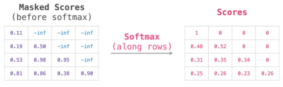
We mask out the words “must obey orders” b/c they happen in the future.
Thus, the softmax’d attention for “robot” is all on “robot”
Forward Pass
- Each decoder has its own weights ($W_q, W_k, W_v$ )
- But entire models shares one token embedding matrix and one positional encoding matrix
Sampling Words
Tune “Top-K” parameter to have GPT-2 consider $K$ most probable words
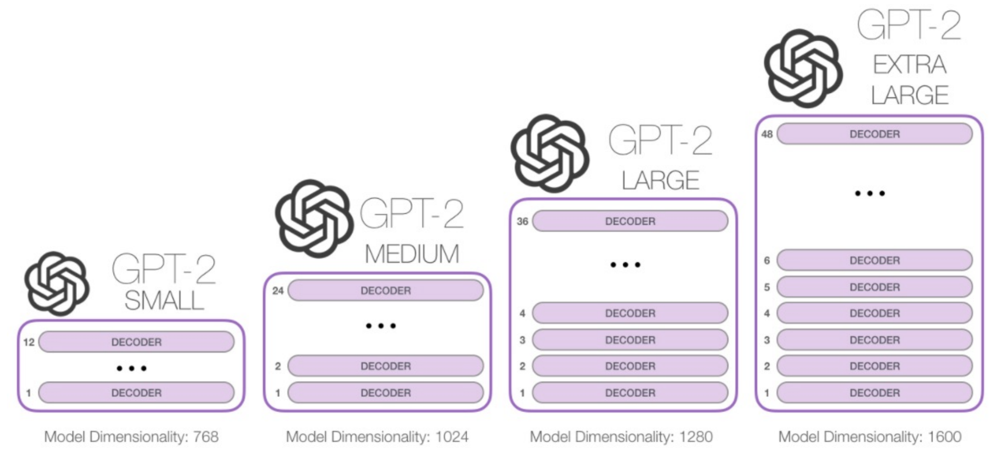
Sizes
Downstream Tasks
Take the learned embeddings from the last layer and add a FFNN to the end of GPT to do downstream tasks:
Machine Translation
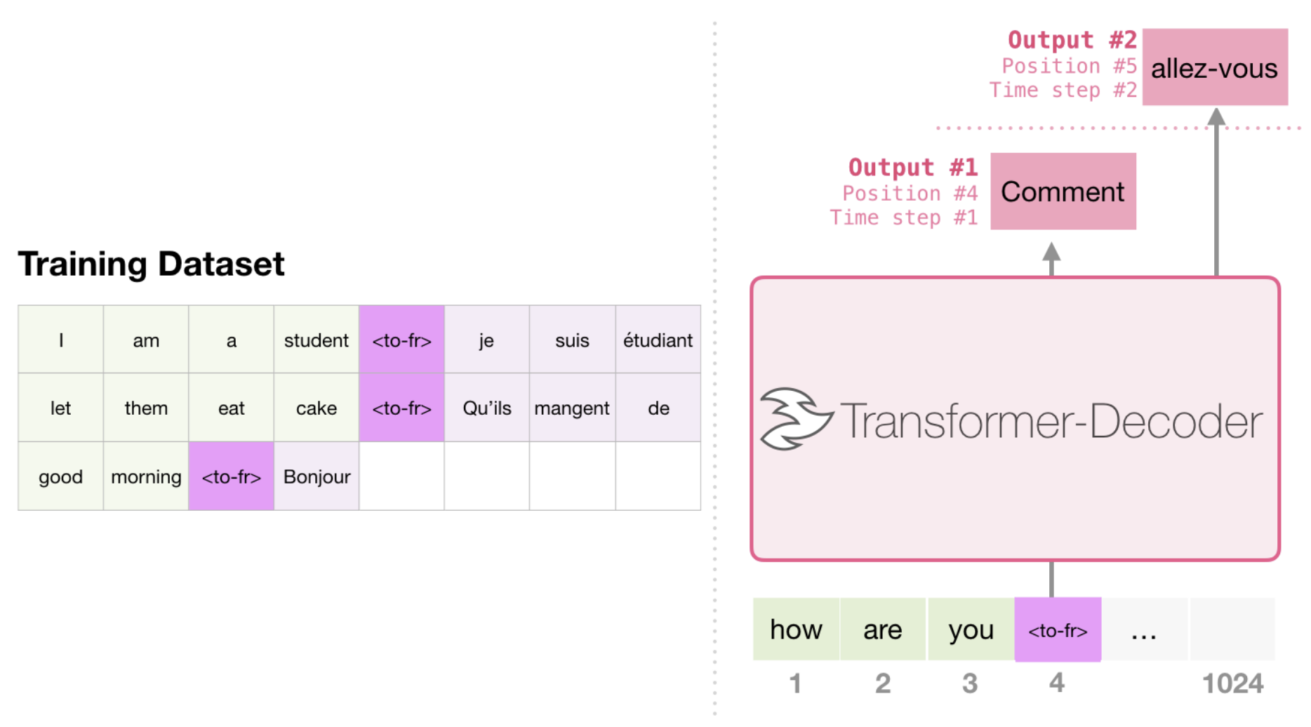
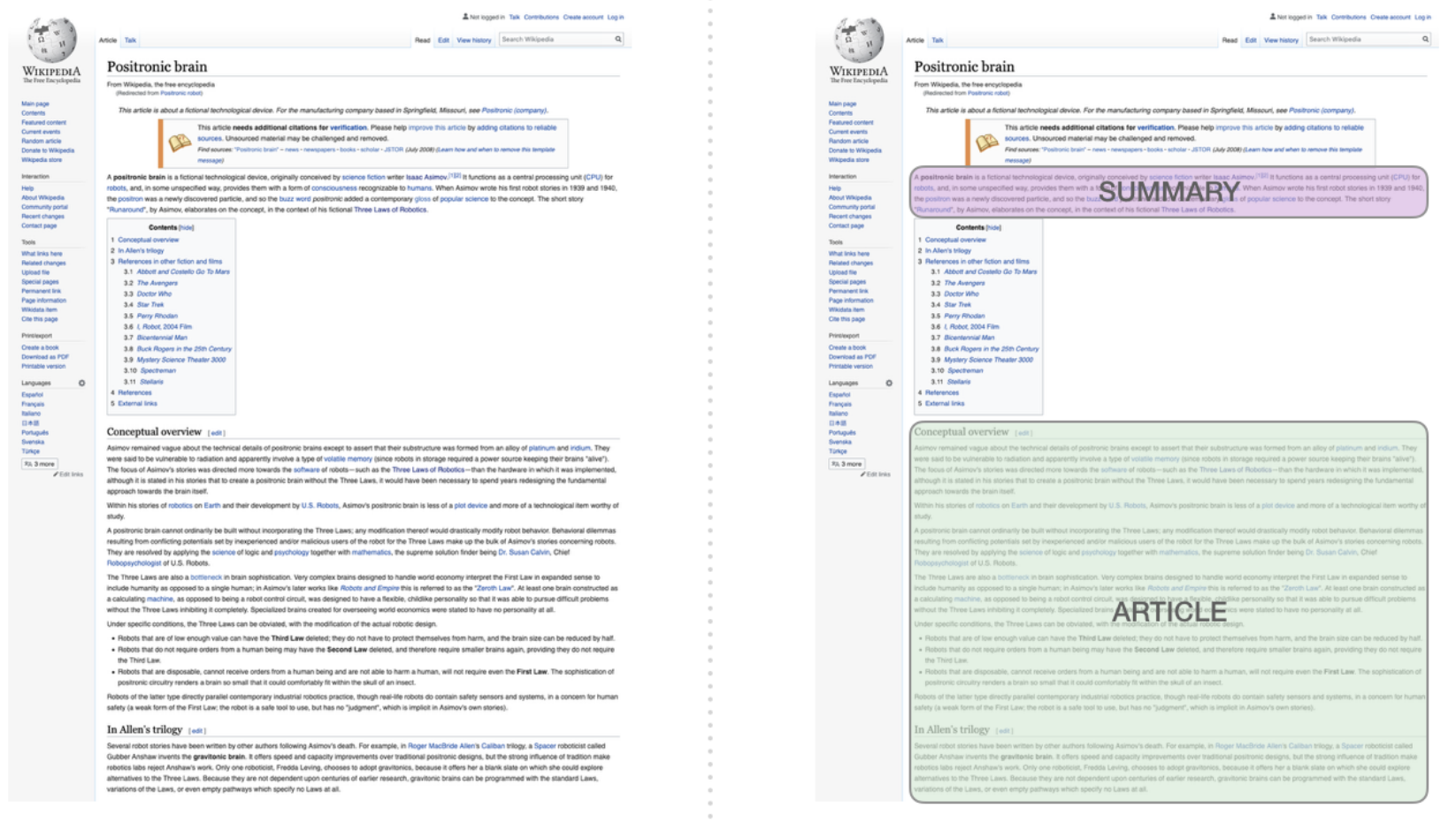
Summarization
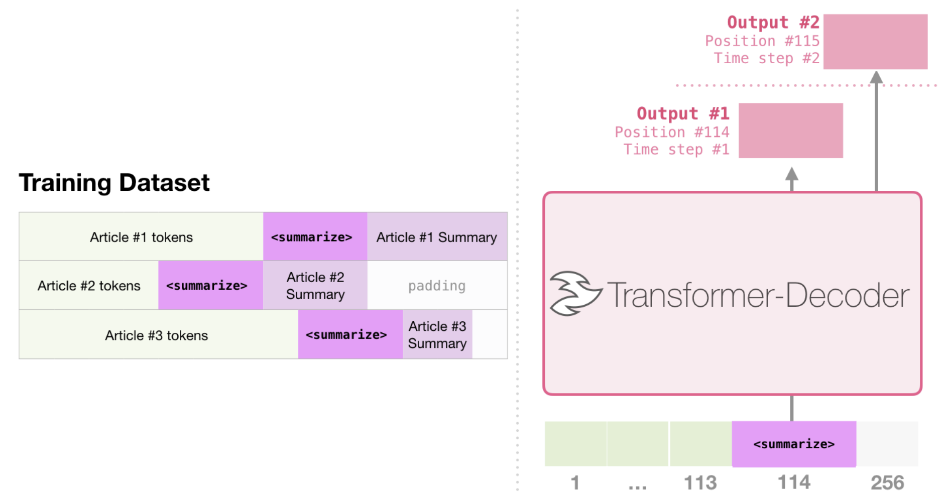
Training data:
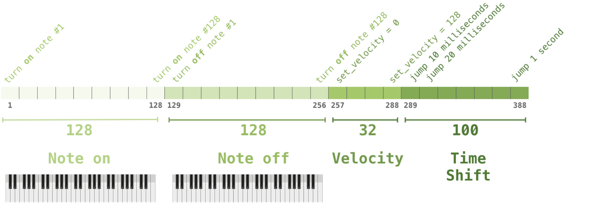
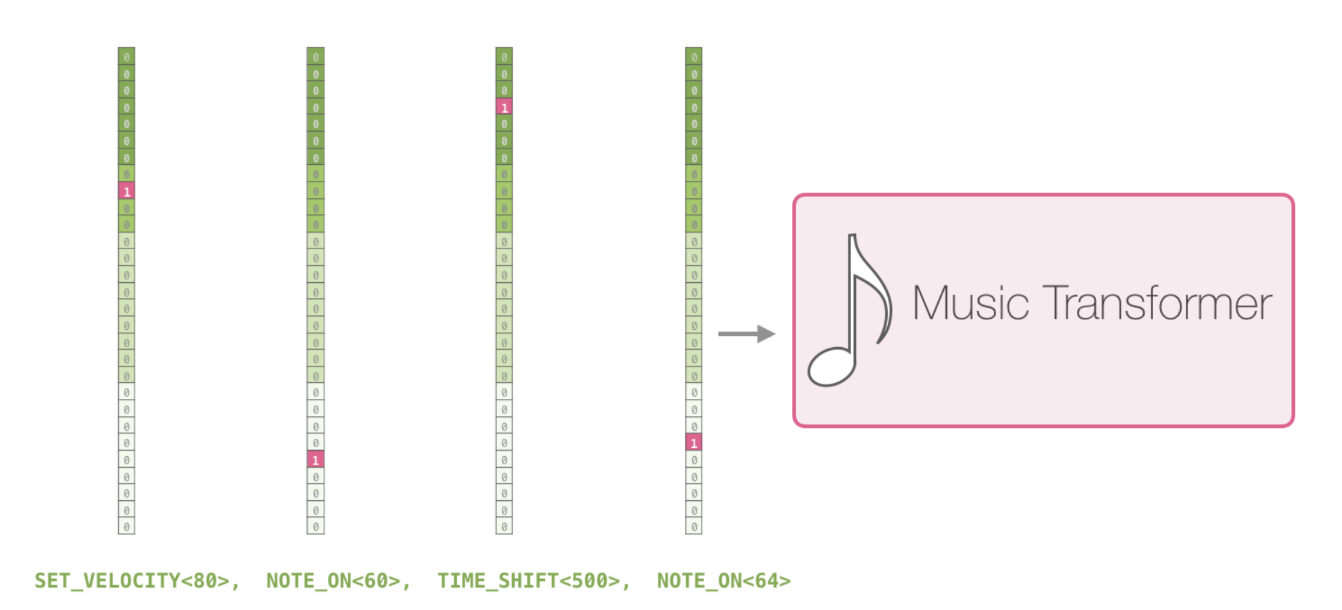
Music Generation
Map musical notes to one-hot vectors, treat musical piece as a sentence of notes, pass through decoder.
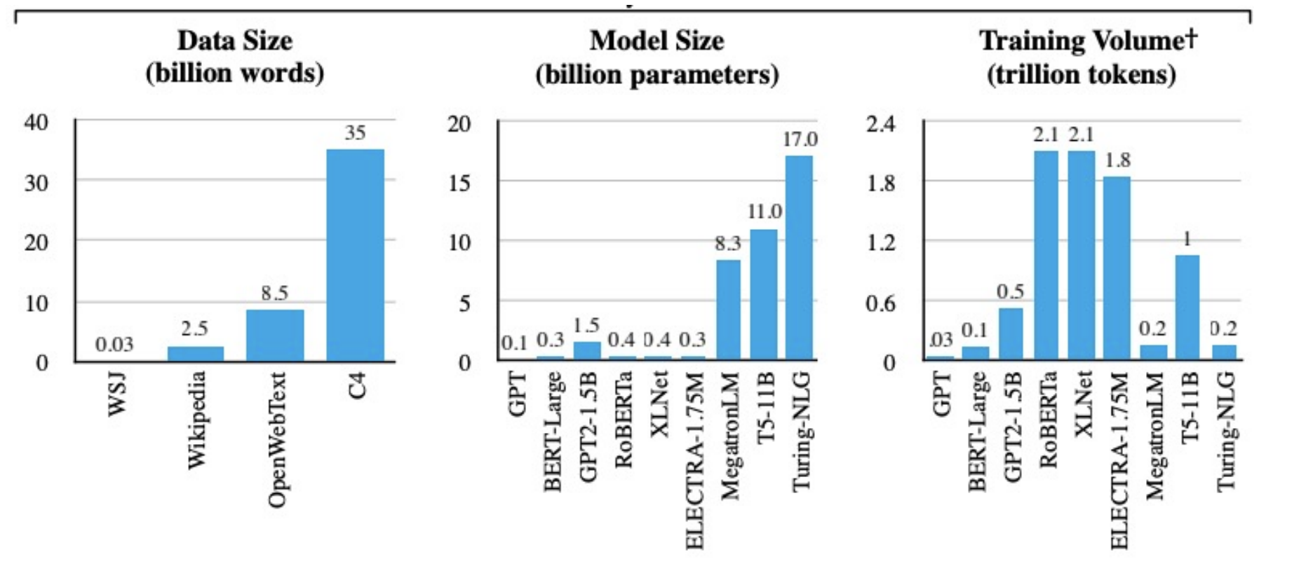
Model Scales
| Model | Dataset | Architecture | # Params |
|---|---|---|---|
| BERT-Base | BooksCorpus (800M words) + English Wikipedia (2.5B words) | 12 transformer blocks + 12 attention heads | 100M |
| BERT-Large | BooksCorpus (800M words) + English Wikipedia (2.5B words) | 24 transformer blocks + 16 attention heads | 340M |
| GPT-2 | 40GB text data | 12-48 decoders | 1.5B |
| GPT-3 | 175B |
Costs
- $2.5 - 50k = 110M params
- $10k - 200k = 340M params
- $80k - 1.6M = 1.5B params
14) Summarization
Types of Input
- Single-doc = Given a single document, produce summary
- Multi-doc = Given multiple documents, produce summary
Types of Output
- Extractive = Select spans from source text that capture key info
- Abstractive = Generate new text to summarize key info
Types of Focus
- Generic = Summarize content of docs
- Query-focused = Summarize with respect to a user’s query (e.g. answer a question by summarizing a doc that has info to construct the answer)
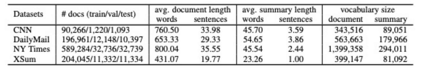
Datasets
These are the most commonly used datasets for summarization NLP tasks:
Metrics
ROUGE-N = (“Recall Oriented Understudy for Gisting Evaluation with $N$ Grams”)
- $n$-gram based comparison motivated by BLEU
- Match machine translation $X$ against $h$ reference human summaries, count total number of $n$-gram overlap between $X$ and $h$ reference summaries
Has very high correlation with human evaluation
Traditional Methods
Steps
- Content selection - choose sentences to extract
- Choose sentences with “salient/informative” words
- tf-idf - weight each word’s informativeness inverse to occurrence
- topic signature - choose a small set of salient words that appear in query
- Weight sentence by average weight of its words
- Choose sentences with “salient/informative” words
- Information ordering - order extracted sentences
- Sentence realization - clean up ordered sentences into a summary
15) Entity Linking (Named Entity Disambiguation)
Task: Identify all named mentions (not nominal mentions) of an entity, and disambiguate them by linking them to nodes in an external knowledge graph (KG)
Two Stage Process:
- Identify mention in text
- Link mentions to entities
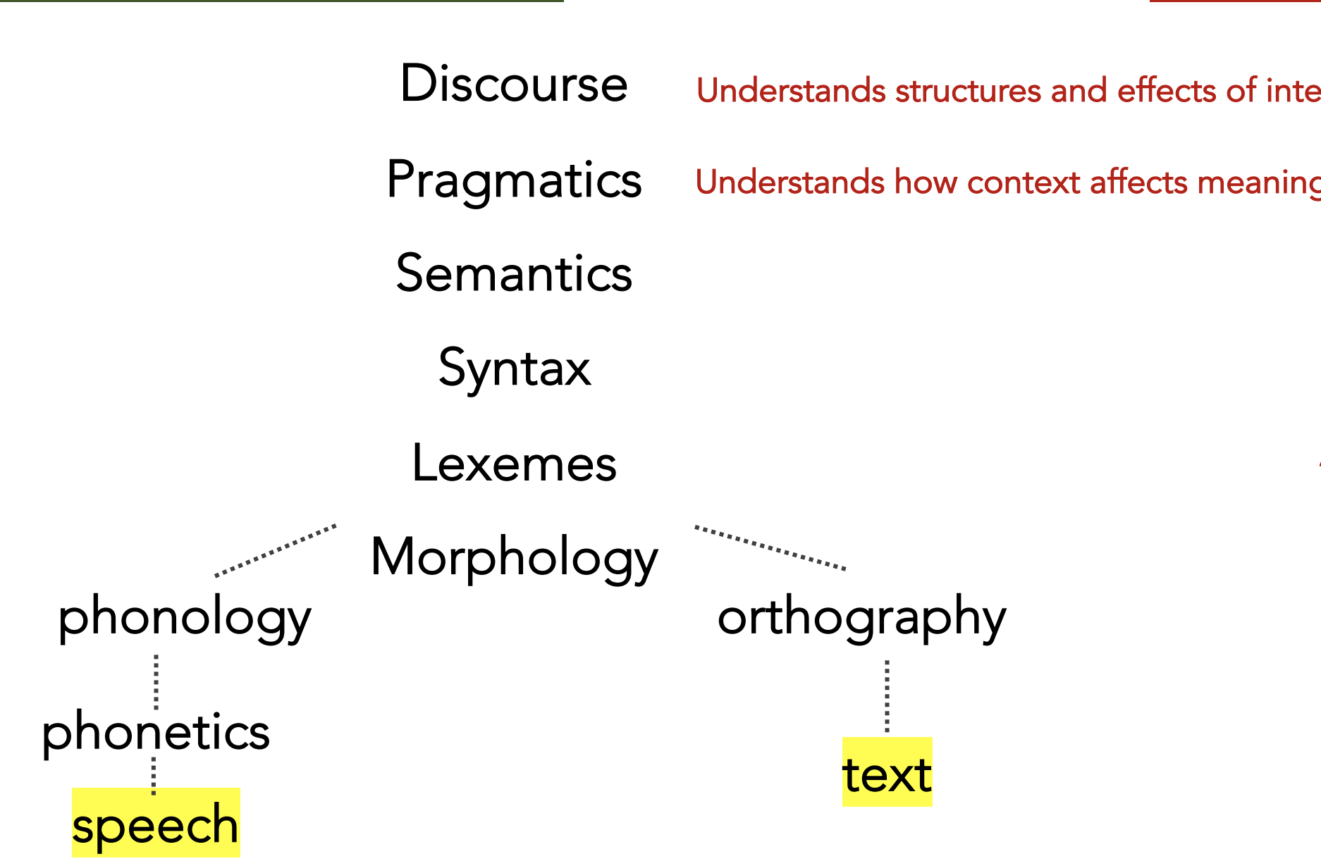
Discourse and Pragmatics
Pragmatics is a branch of linguistics dealing with language use in context (non-local meaning phenomena)
Datasets
- TACKBP-2010
- 2k annotated mention/entity pairs
- Linked to TAC Reference Knowledgebase w/ 818k entities
- AIDA/CoNLL
- 26k annotated mention/entity pairs
Metrics
- Disambiguation-only
- Micro-precision = % of correctly disambiguated entities in full corpus
- Macro-precision = % of correctly disambiguated entities, averaged by doc
- End-to-end approaches
- Micro-F1 =
- Macro-F1
- Recall @ N
- Accuracy
Baselines
Link popularity
- Build dictionary of name variants for each entity
- Inspect all KB entities that have a name variant which matches the query mention
- Choose the entity w/ highest # of inlinks with query
TODO
XXXX
End-to-End DL Approach
TODO
16) Coreference Resolution
This section was taken directly from: https://web.stanford.edu/~jurafsky/slp3/21.pdf
Task: Determine which words refer to the same real-world entity (basically a clustering task)
Evaluation: Given text $T$, find all entities + coreference links between them. Compare our graph to a goldstandard human-annotated graph for $T$.
- Lack of singletons in evaluation set makes task easier, b/c singletons are harder to detect
- Identify mentions of entities
- Cluster discourse entities into set of coreferring expressions (aka “coreference chains” or ““clusters”)
- Link discourse entities to real-world entities via ontologies
In below excerpt, superscripts corefer to the same entity
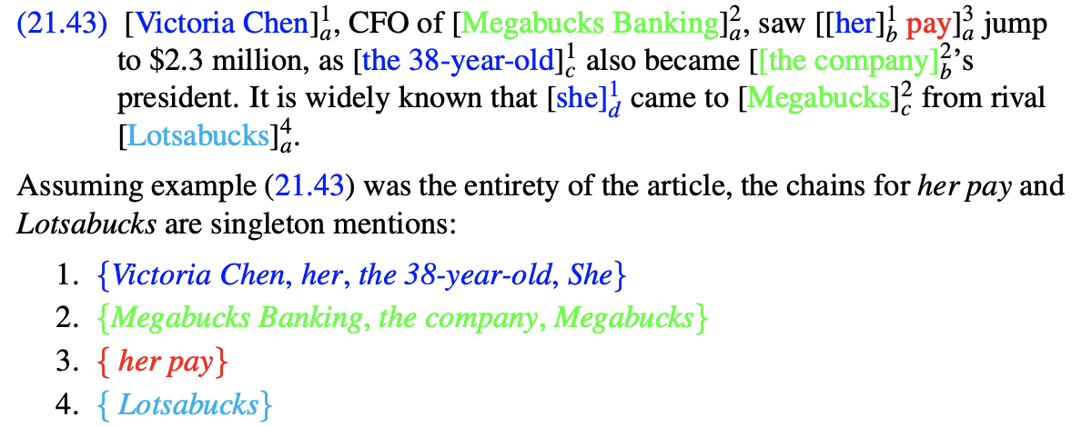
Terms
Anaphor = expression that references a previously mentioned entity
Antecedent = entity that anaphor references
Singleton = entity with only one mention (e.g. no antecedent)
Linguistic Background
Types of referring expressions:
- Indefinite Noun Phrases (NPs)
- “a XXXX”
- Introduces a new entity to the hearer
- Definite NPs
- “the XXXX”
- References a previously mentioned entity or entity already known to the hearer (e.g. “the USA”)
- Pronouns
- Pronouns: “he/she/it/they”
- Demonstrative: “this/that/these/those”
- Names
- “IBM/John Smith/New York”
Information status of referring expressions:
- New NPs
- Introduce new entities into discourse
- Old NPs (“evoked NPs”)
- Entities already in discourse
- Inferrables
- Can be inferred from prior in the conversation to exist via a “bridging inference”
- e.g. “I went to a restaurant yesterday. The chef had just opened it.”
Non-referring expressions:
- Appositives
- Sometimes counted as a coreferential (e.g. OntoNotes) even though describe head NP rather than corefer to it
- e.g. “Victoria, CFO of Megabucks, saw that…”
- e.g. “United, a unit of UAL, matched the fares…”
- Predicative and Prenominal NPs
- Describe properties of a head entity, rather than referring to that distinct entity
- e.g. “United is a unit of UAL”
- e.g. “her pay jumped to $2.3 million”
- Expletives
- Pronouns that don’t refer to anything
- e.g. “It was Emma who founded the company.”
- e.g. “We hit it off”
- Generics
- Expression that doesn’t refer back to the entity explicitly referencing it in the text
- e.g. “I love mangoes. They are tasty.”
Properties of coreference relationship:
- Number agreement
- Referring expresions and referents must usually agree in number (e.g. “she” v. “they”)
- Person agreement
- 1st/2nd/3rd person – e.g. “I” v. “he” v. “you”
- Gender or noun class agreement
- e.g. “John is great. He is awesome.”
- Binding theory constraints
- e.g. “Jane bought herself a bottle of sauce.”
- Recency
- e.g. “Sally doctor found an old map in the captain’s chest. Jim found an even older map hidden on the shelf. It described an island.”, where it refers to Jim’s map
- Grammatical role
- Entities in subject are more salient than object which are more salient than oblique references
- Verb semantics
- e.g. “John called Bill. He had lost the laptop”. He refers to John
- e.g. “John criticized Bill. He had lost the laptop.” He refers to Bill
Process
- Mention detection
- Emphasizes recall
- Run parser that identifies every NP, pronoun, or named entity
- Run anaphoricity detector on parsed entities
- Only keep anaphoric mentions
Models
Two approaches:
- Entity-based – represent each entity in discourse model
- Mention-based – consider each mention independently
Mention-Pair Architecture
- Input: (anaphor, antecedent)
- Output: 1 if coreferring, 0 else
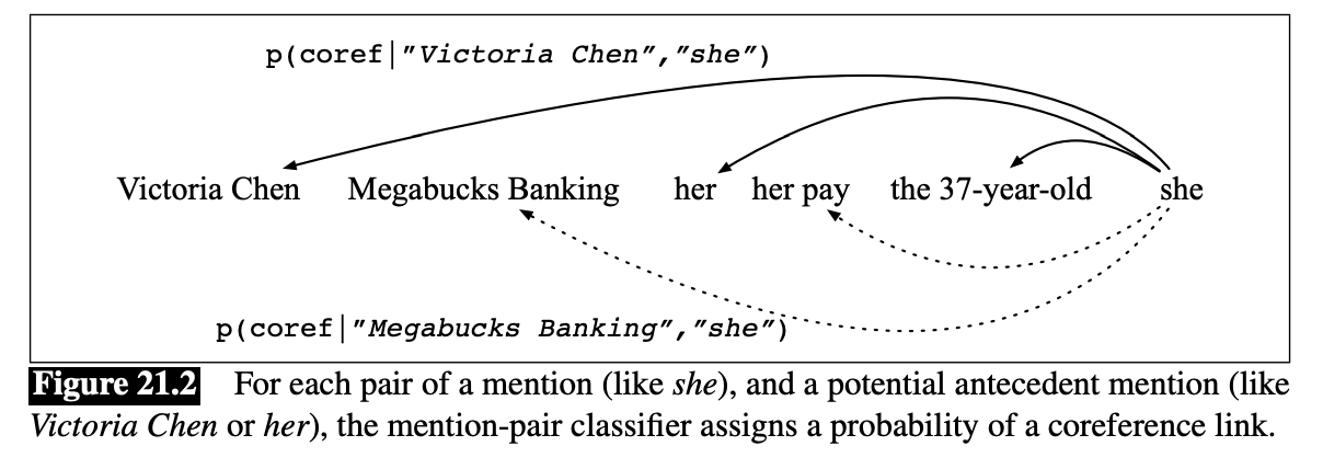
- Training sample selection strategy:
- Choose closest antecedent as (+) example
- All pairs between as (-) examples
- Avoids flooding traing set with (-) examples
- Evaluation on test set:
- For each mention $i$ in document, consider each of prior $i-1$ mentions
- Closest-first clustering – run classifier from $i-1$ to 1, and first antecedent with prob > 0.5 is linked to $i$
- Best-first – run classifier from $i-1$ to 1, antecedent with highest overall prob is linked to $i$
Problems:
- Doesn’t directly compare candidate antecedents
- Ignores discourse model
- Only considers local pairwise info
Mention-Rank Architecture
Idea: Directly compare candidate antecedents
For the $i$th mention (anaphor), we have a rv $y_i \in {1, …, i-1, \epsilon }$ where $\epsilon$ means there is no antecedent
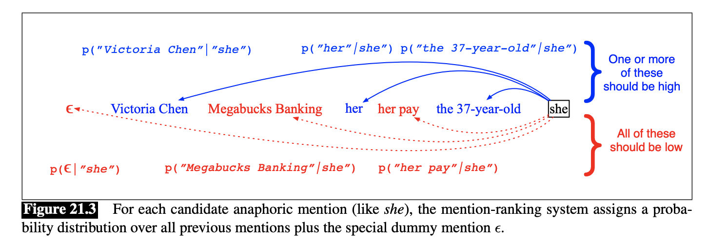
- Training sampling strategy:
- Need to choose which of possible legal gold antecedents to train on – instead, can just sum over probability assigned to all legal antecedents
- Evaluation on test set:
- Compute one softmax over all antecedents (and $\epsilon$)
Entity-based Models
Idea: Instead of linking mentions to previous mentions, link them to previous entities (i.e. clusters of mentions)
- Can turn a mention-ranking model -> entity-ranking model by having the classifier make decisions over clusters of mentions rather than individual mentions
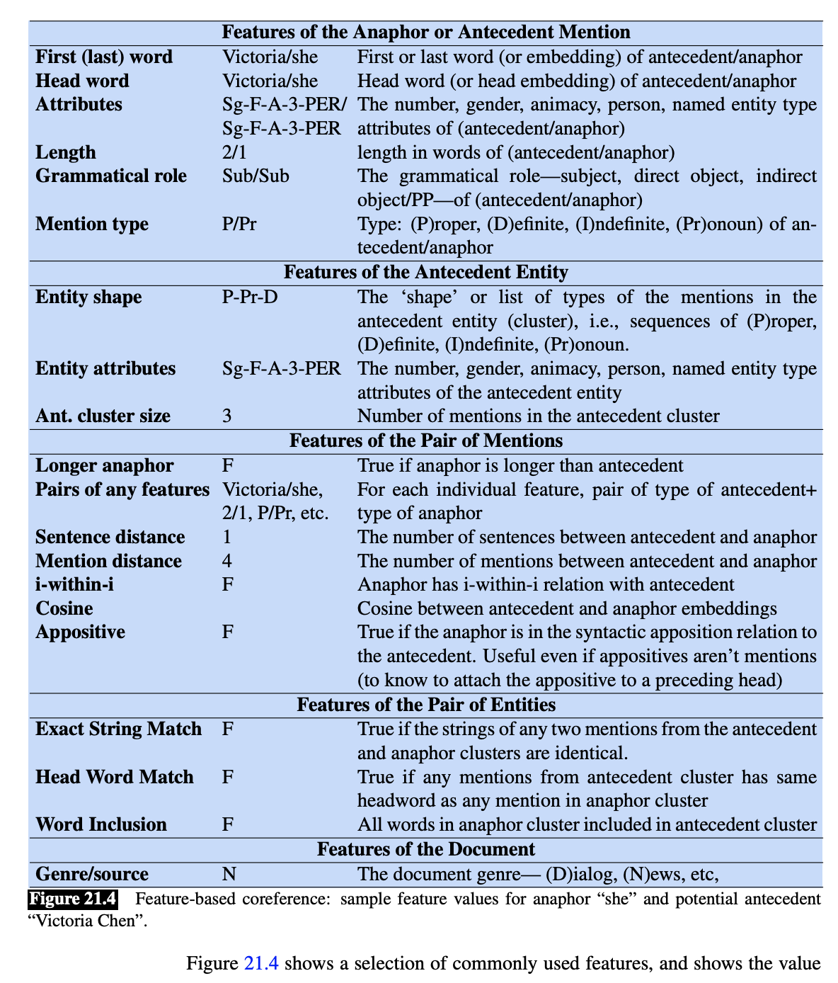
Features
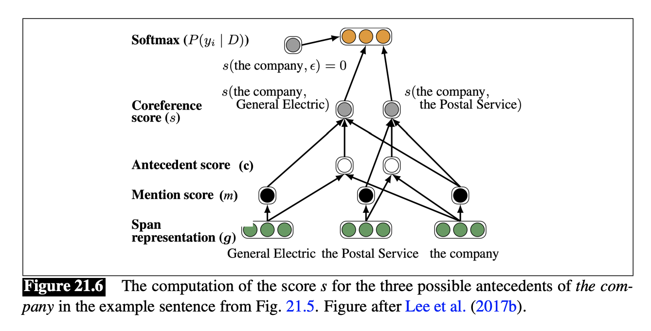
e2e-coref Model
-
Mention-ranking algorithm
-
Given document $D$ with $T$ words, considers all $n$-grams up to size $n \le 10$
-
Task: Assign each span $i$ an antecedent $y_i \in {1, …, i - 1, \epsilon }$.
-
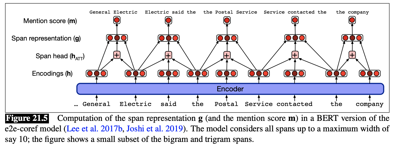
For each pair of spans $i,j$, assign a score $s(i,j)$ for the coreference link between $i$ and $j$.
-
$P(y_i) = softmax(s(i, y_i))$
-
where
-
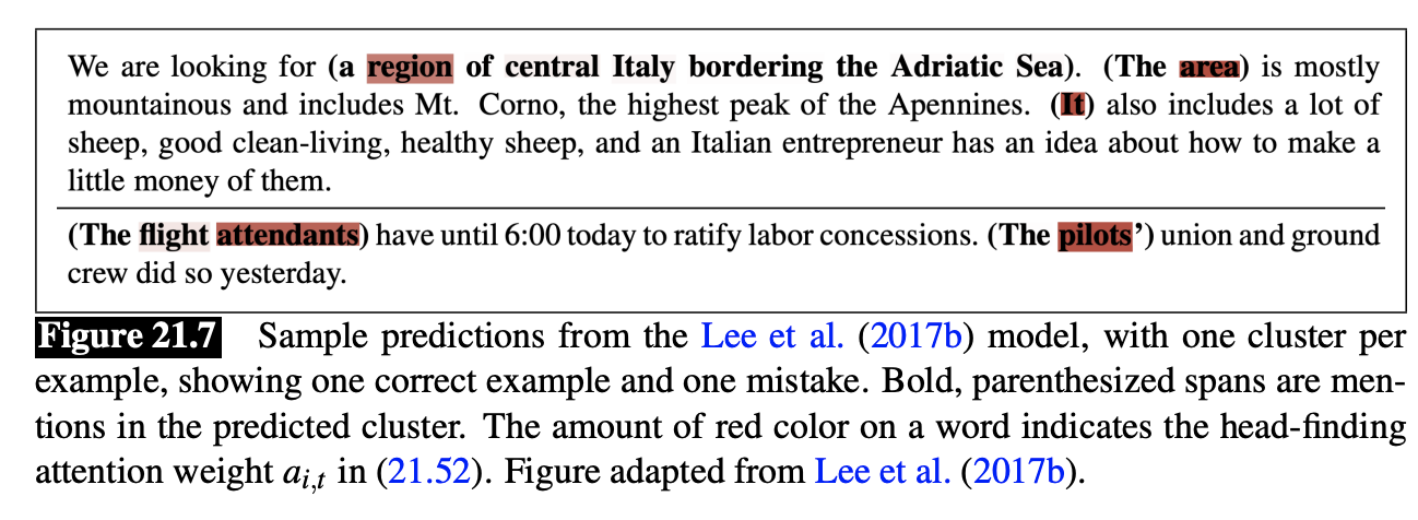
$s(i,j) = m(i) + m(j) + c(i,j)$
-
$m(i)$ = 1 if $i$ is a mention
-
$m(j) = 1$ if $j$ is a mention
-
$c(i,j)$ = 1 if $j$ is antecedent of $i$
-
and $s(i, \epsilon) = 0$ is fixed
-
-
We define:
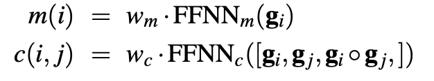
To generate span representations $g_i$:
- Run each paragraph through BERT to generate embedding $h_i$ for each token $i$
- Define $h_{att}$ as the likely head-word of the span, $h_{start/end}$ as the start and end word of the span
- Each span $g_i$ is:
- $g_i = [ h_{start}, h_{end}, h_{att} ]$
Datasets
- OntoNotes
- Hand-annotated Chinese + English of ~1M words each + 300k words of Arabic newswire
- No labels for singletons (which are ~70% of all entities)
- ISNotes - portion of OntoNotes annotated for info status
- LitBank = 210k tokens from 100 novels (includes singletons)
- ARRAU = 350k English words (includes singletons)
- Diverse genre of content
- ECB+ = 982 short documents on “event coreference”
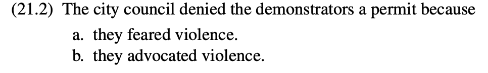
- Example:
- Example:
- Winograd
- Example:
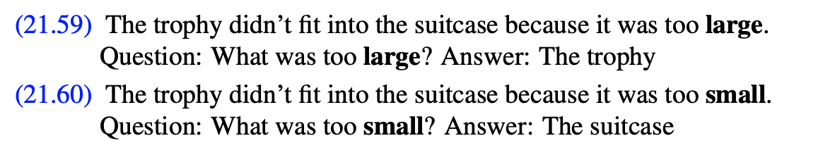
- Example:
- Example:
- WinoBias
- Example:
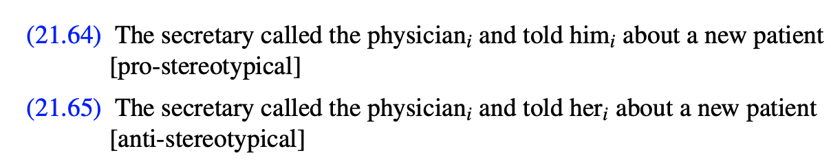
- Example:
Evaluation + Metrics
Model outputs series of clusters $H$ v. gold standard set of clustesr $R$
- MUC F-Measure
- Link-based
- Based on # of coreference links (i.e. pairs of mentions) common to $H$ and $R$
- Precision = # of common links / # of links in $H$
- Recall = # of common links / number of links in $R$
- CONs
- Biased toward models that produce large chains
- Ignores singletons
- B^3
- Mention-based
- Given mention $i$, the set of correct mentions in $H_i$ is $H_i \and R_i$
-
Precision = $\frac{ H_i \and R_i }{H_i}$ -
Recall = $\frac{ H_i \and R_i }{R_i}$
-
- Total precision/recall = weighted sum of precision across all mentions in $R$
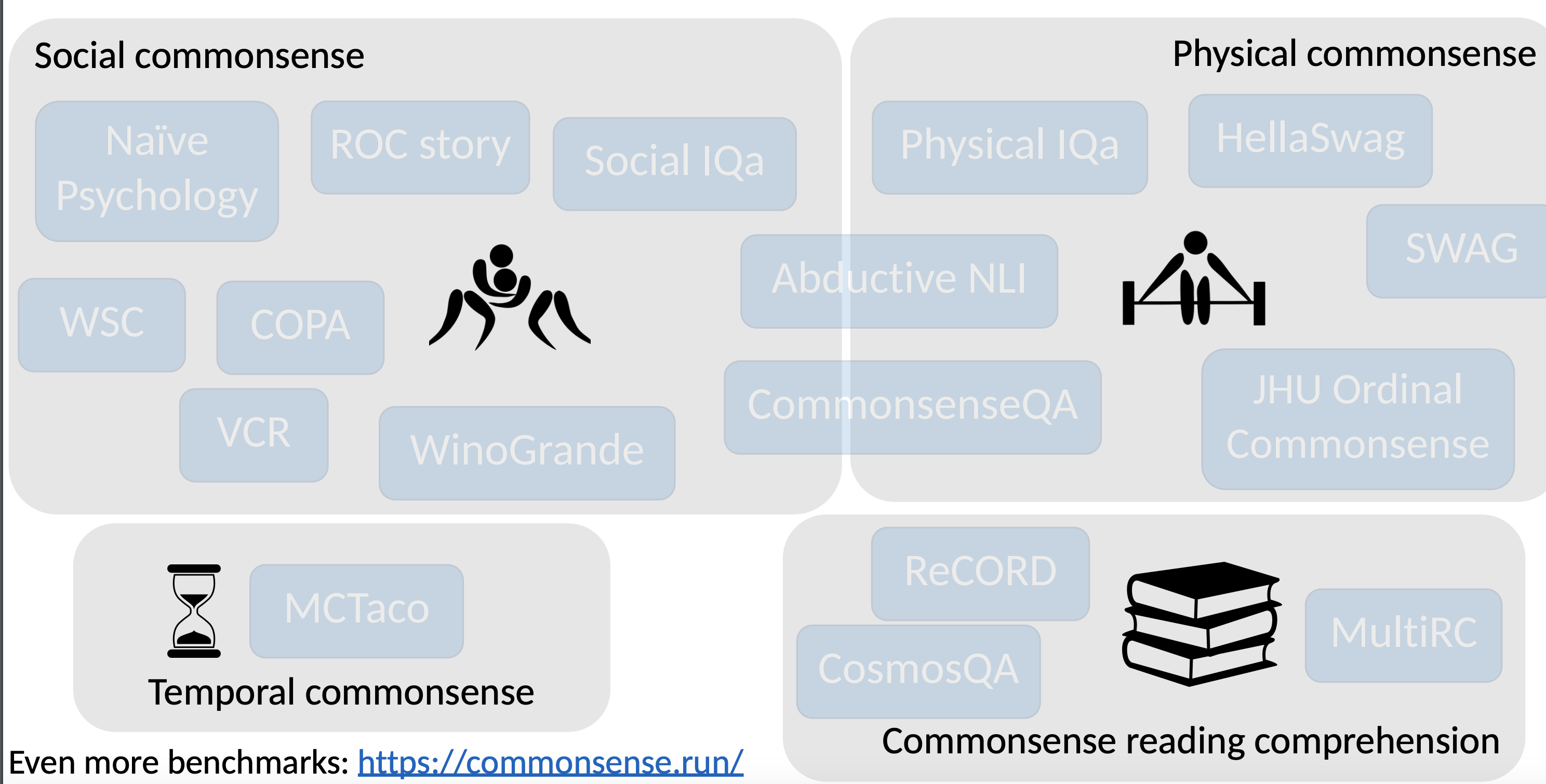
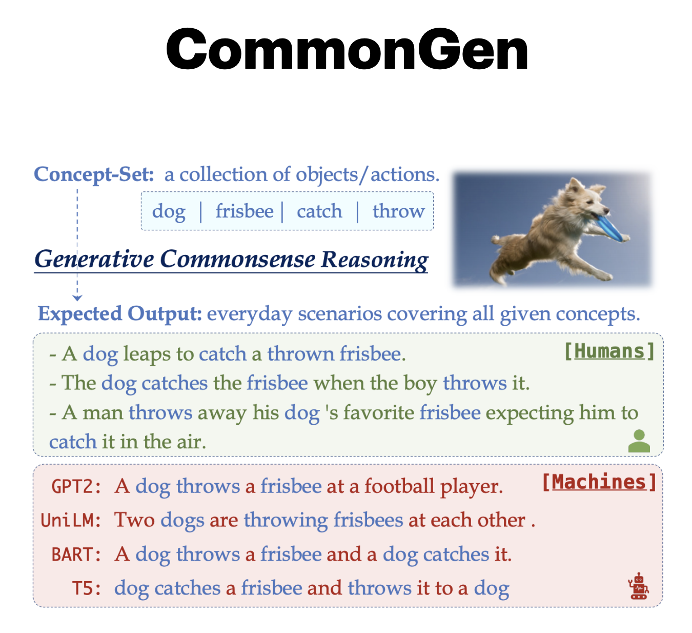
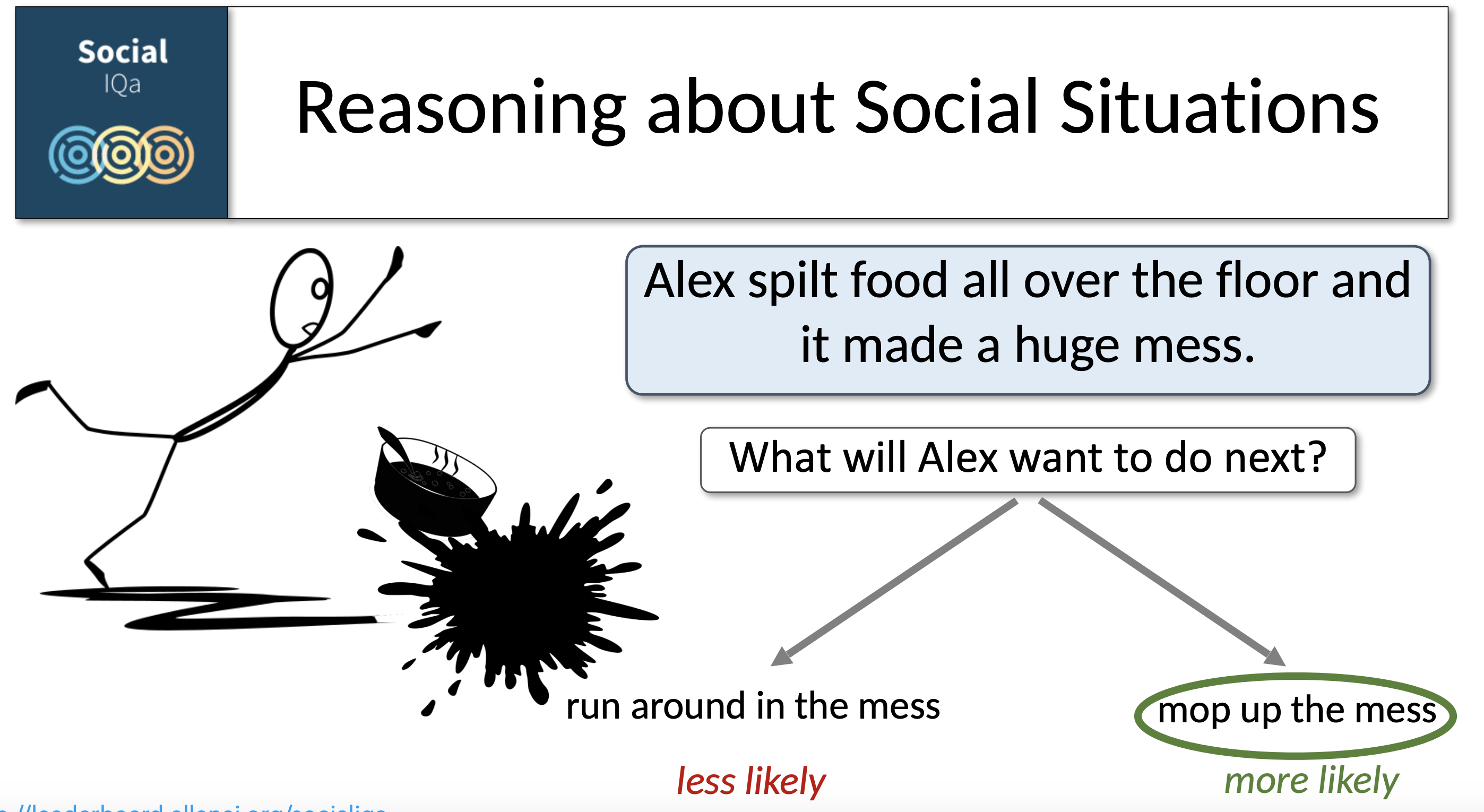
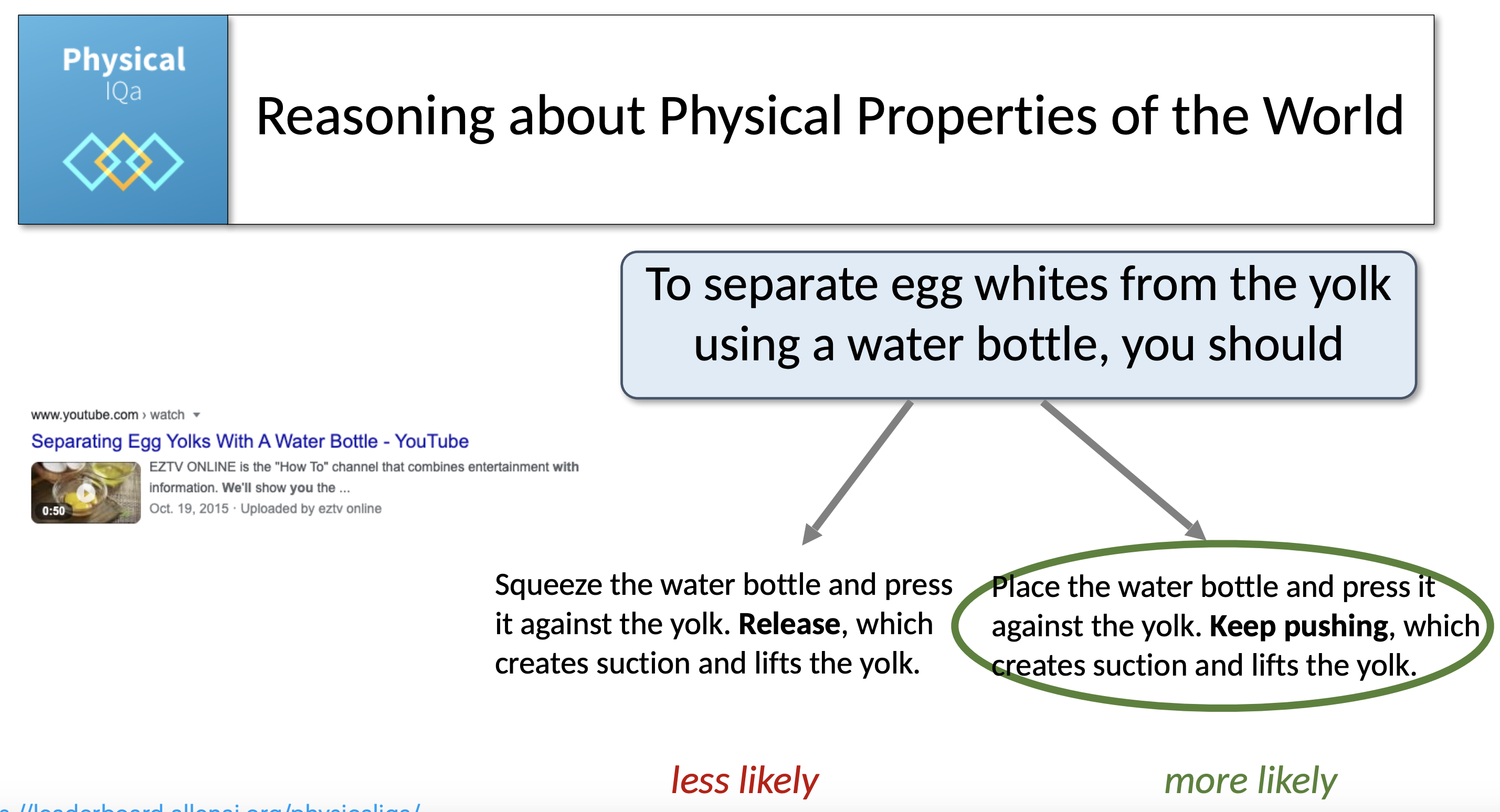
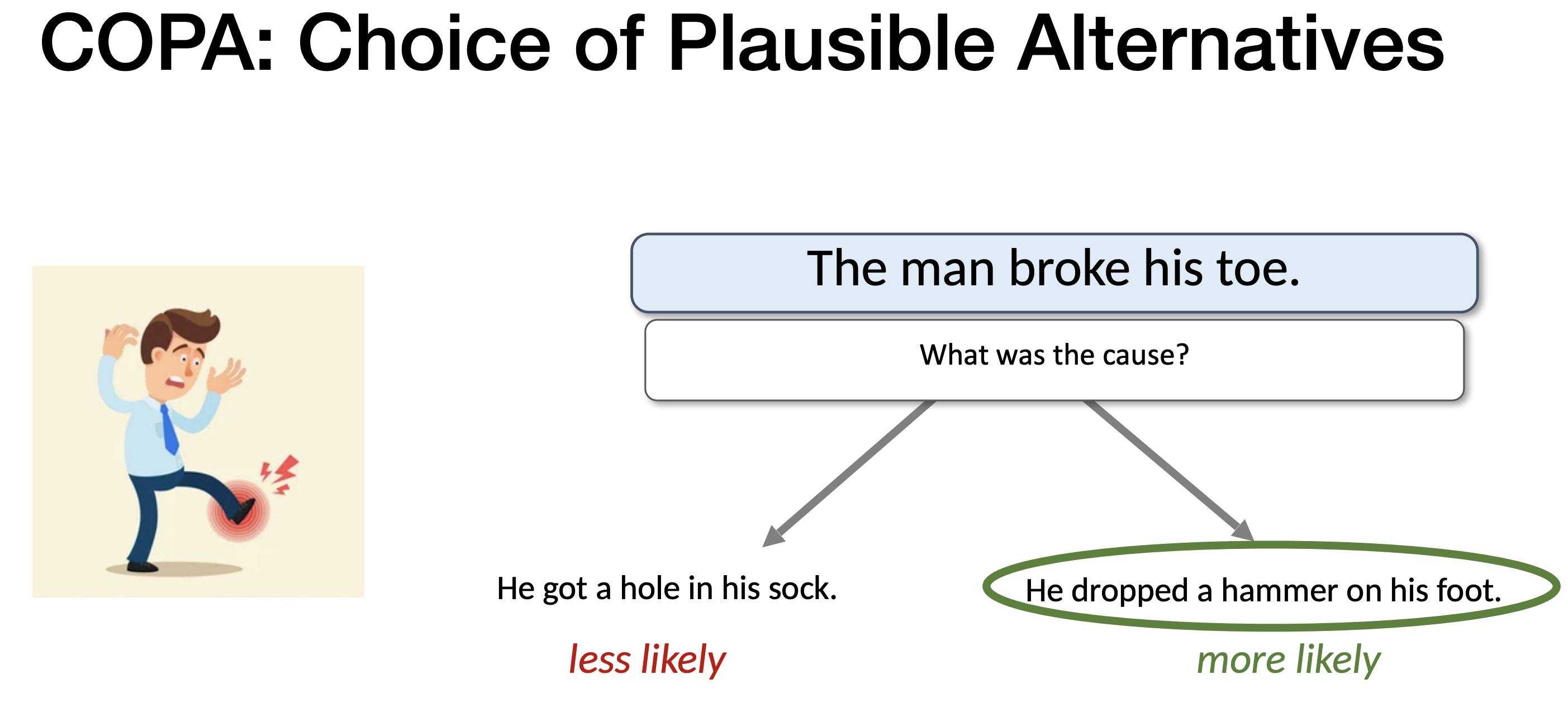
17) Common Sense
Datasets
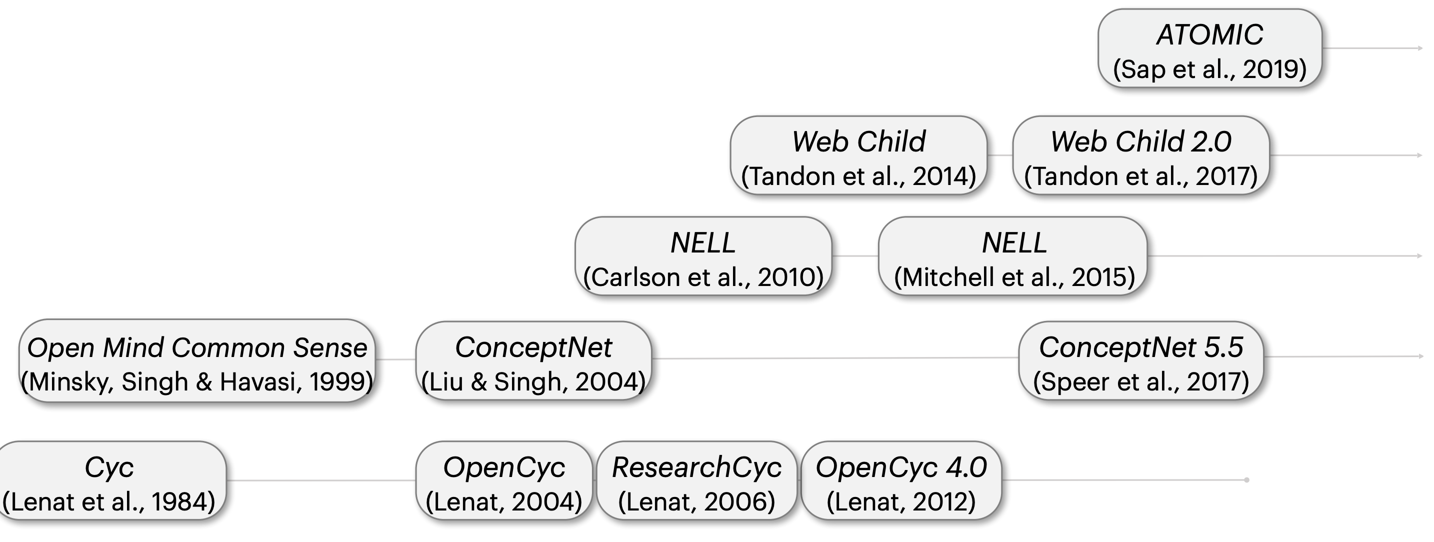
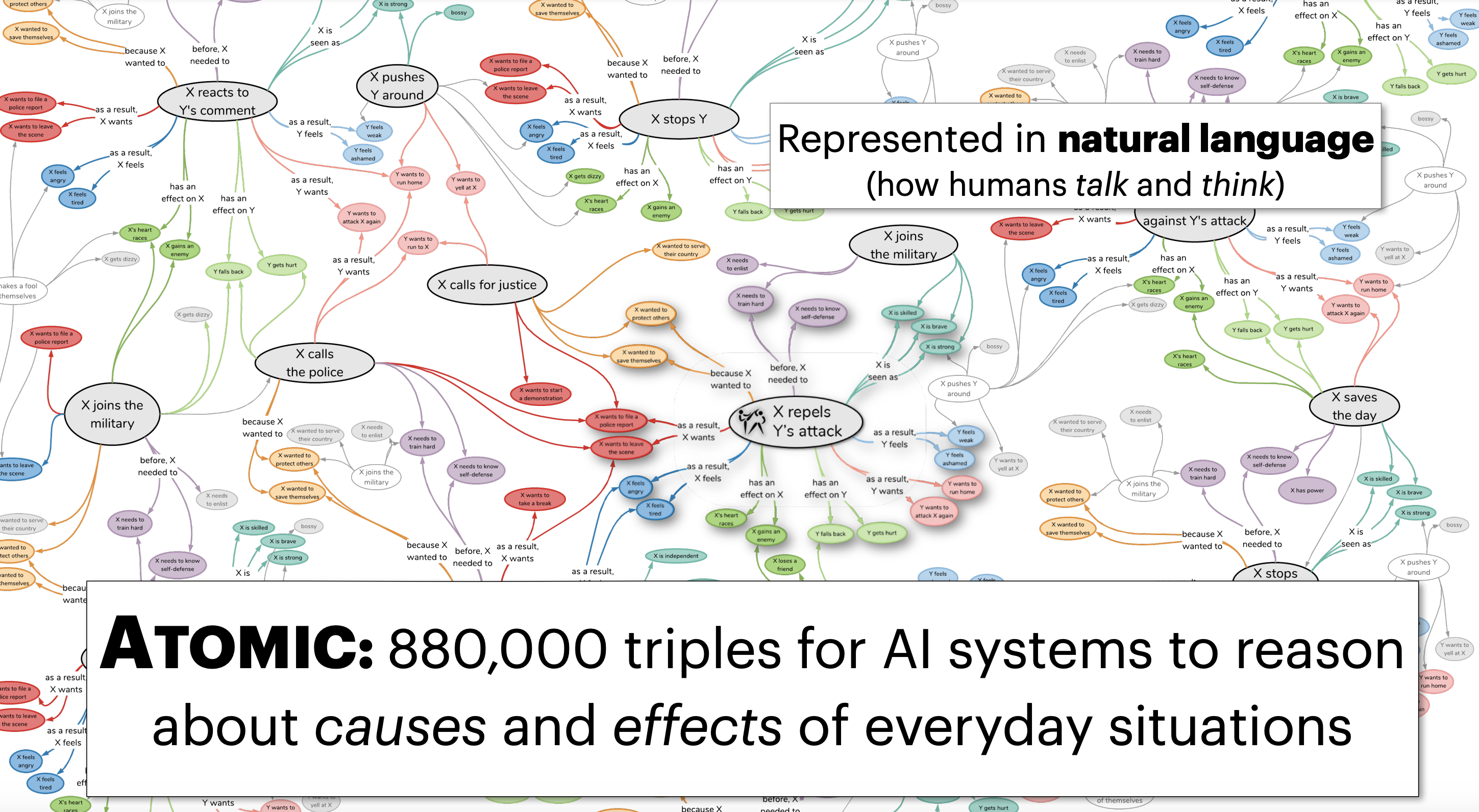
Knowledge Bases
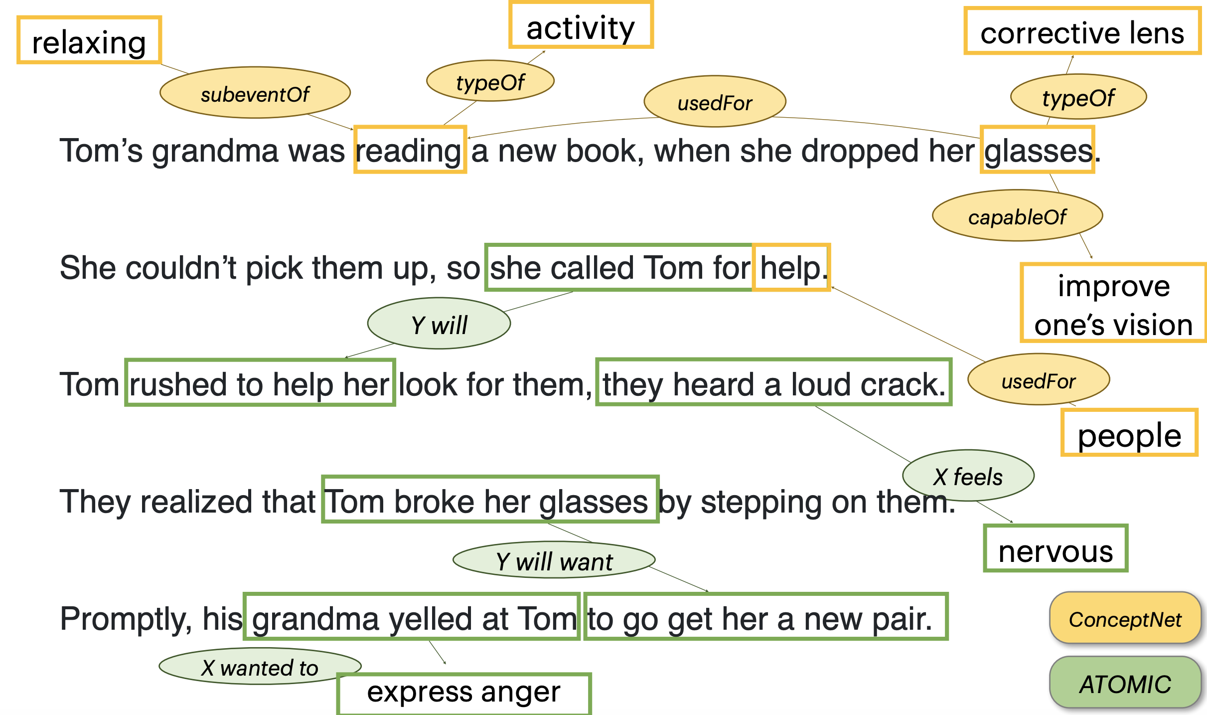
Models
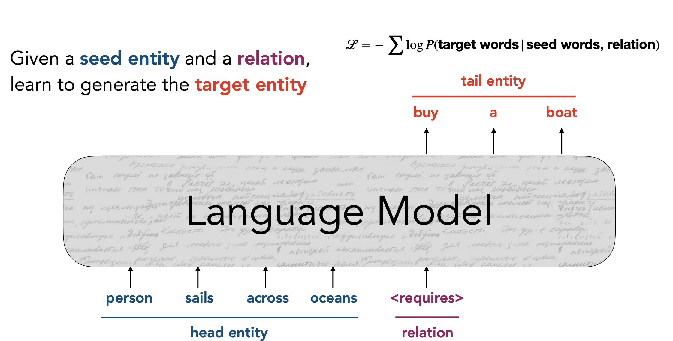
COMET = Common Sense Transformer model
- Generate commonsense knowledge for any input concept using a language model
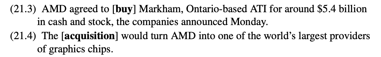
- Input: (Head entity, relation)
- Output: (Target entity)
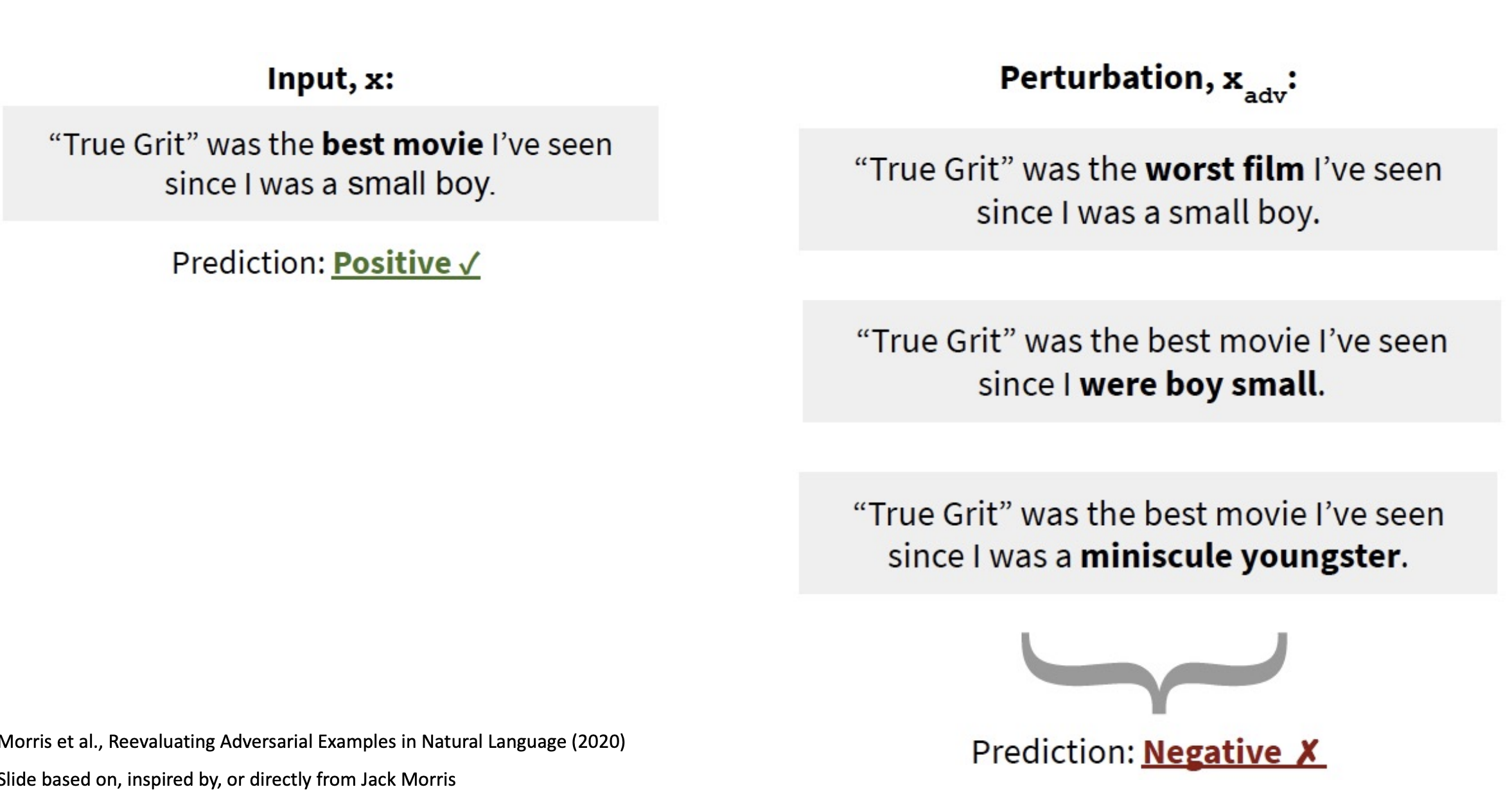
18) Adversarial NLP
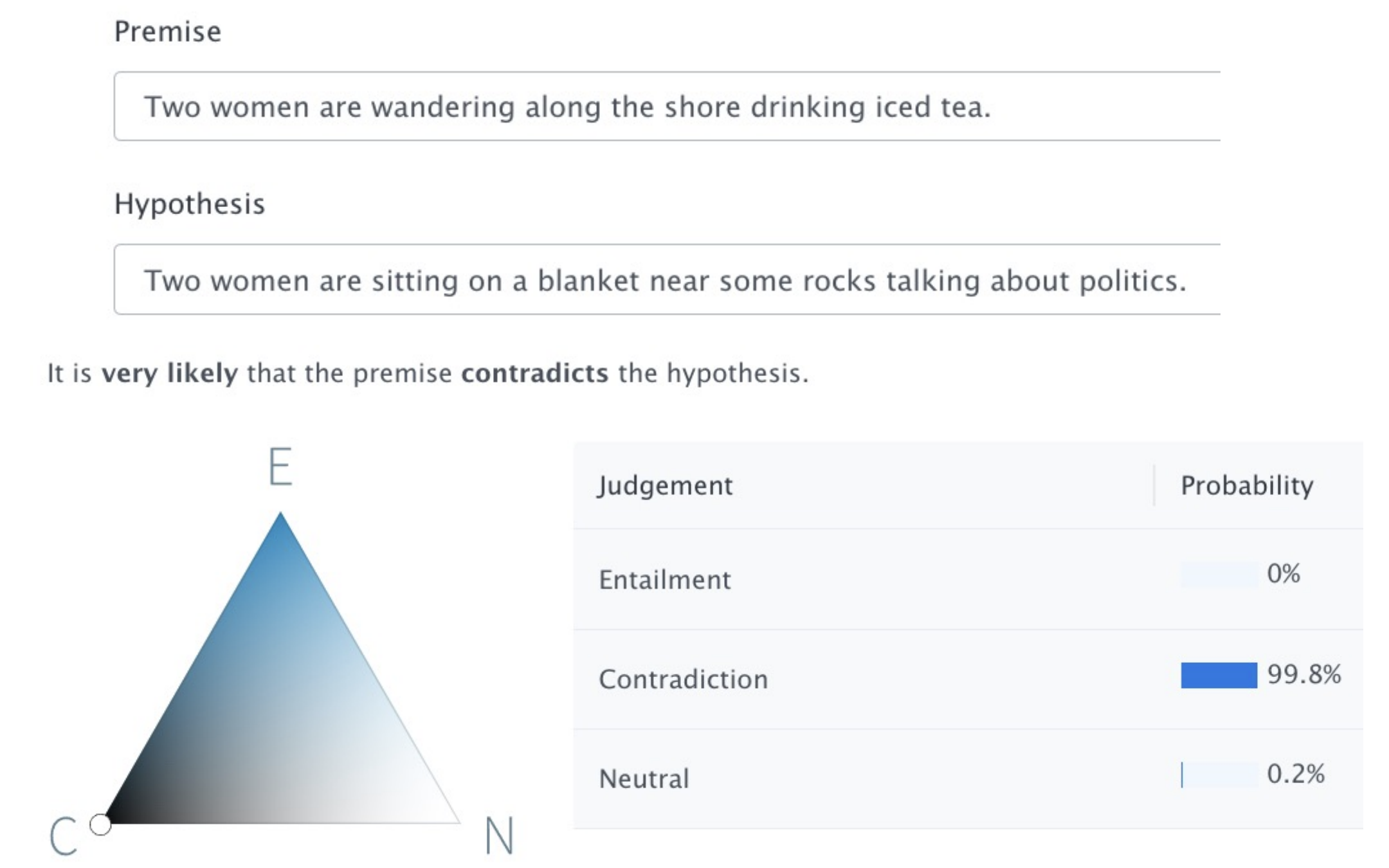
Textual Entailment = Task of predicting whether facts of Sentence 1 necessarily imply facts of Sentence 2
Threat Model
Let $(x,y)$ be (input, output) and $x’$ be an altered version of $x$ which yields $y’$
| Successful attack minimizes $ | x - x’ | $ while maximizing $ | y - y’ | $ to get $class(y) \ne class(y’)$ |
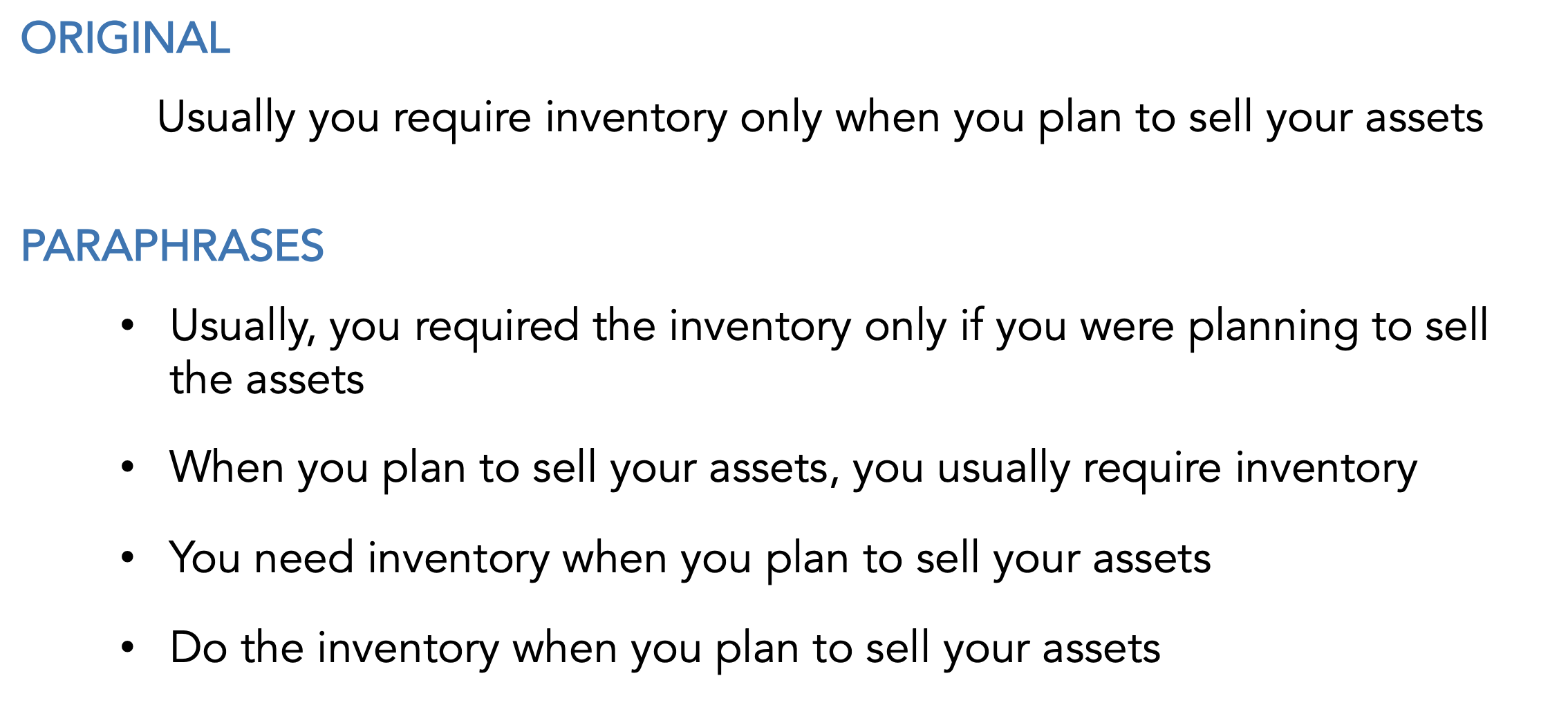
Paraphrasing
How can we change text while preserving its meaning?
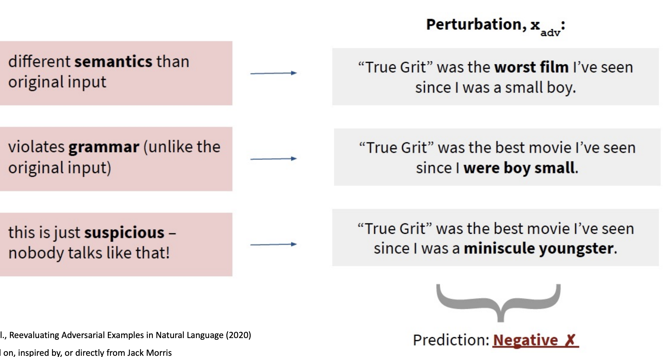
Word-Level Substitutions (aka lexical)
Substitute synonyms at the word level to preserve sentence meaning.
- Embeddings - Search for nearest-neighbor in embedding space
- Thesaurus - Lookup word in thesaurus, WordNet, PPDB
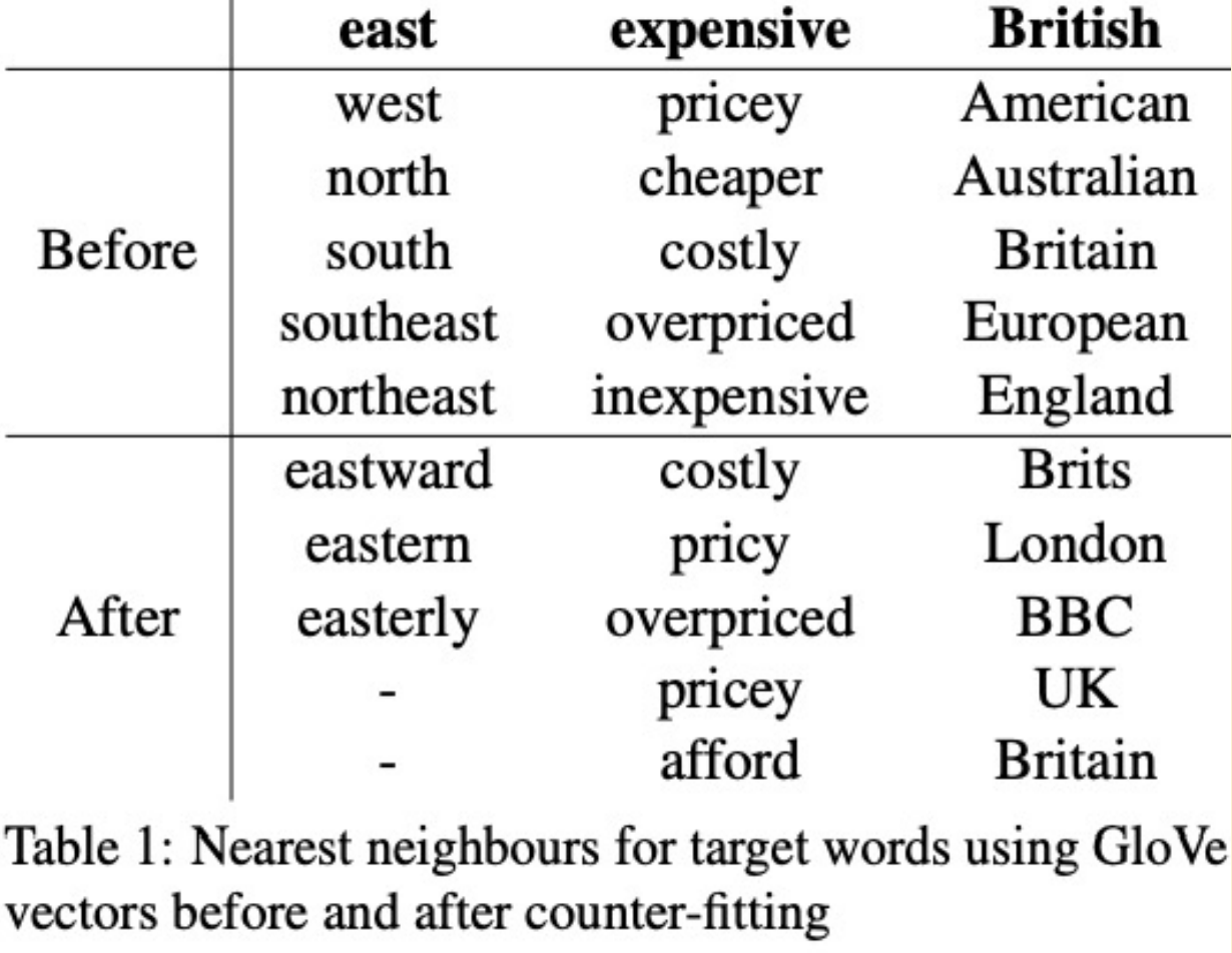
- Hybrid - Search for nearest-neighbors in “counter-fitted” embedding space
- Inject antonymy + synonymy constraints into vector space representations
- Separates conceptual association from semantic similarity
Sentence-Level Substitutions (aka syntactic)
Goal: Get adversarial inputs that are grammatical, preserve input semantics, have minimal lexical substitution, and high syntactic diversity
- Cosine similarity btwn $x$ and $x’$ sentence embeddings
- Substitute phrases (PPDB)
- Machine translation
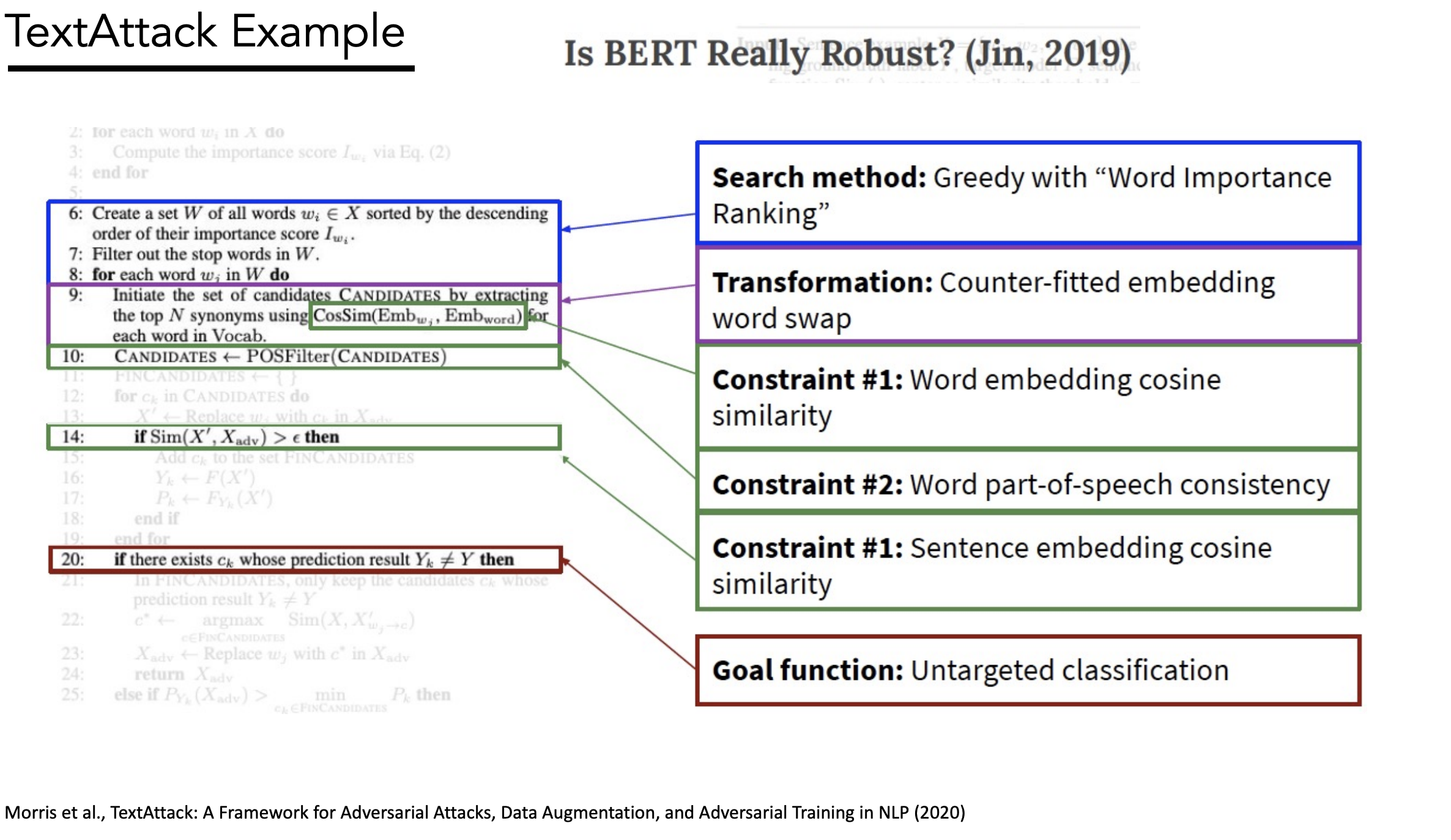
“TextAttack” Framework
Checklist for adversarial attacks
- Goal function - determines whether attack is successful
- e.g. minimum BLEU score
- Constraints - determine if perturbation $x’$ is valid w/ respect to original input $x$
- e.g. max word embedding distance
- Transformation - generates perturbation $x’$ from $x$
- e.g. thesaurus word swap
- Search method - select promising $x’$ by querying model
- e.g. beam search
19) Debugging
Training
- Is loss function going down?
- Is loss going to 0 after running for long enough?
- Is loss going to 0 using a small training set?
Deliberately try to overfit. If not, error.
Model Size
Try increasing model size.
Larger models learn with fewer steps

Optimization
- Optimizer - Adam or SGD?
- Learning rate - Standard or decay?
- Initialization - Uniform or Glorot?
- Minibatch - Large enough batch?
Beam search
Longer $K$ should yield better performance
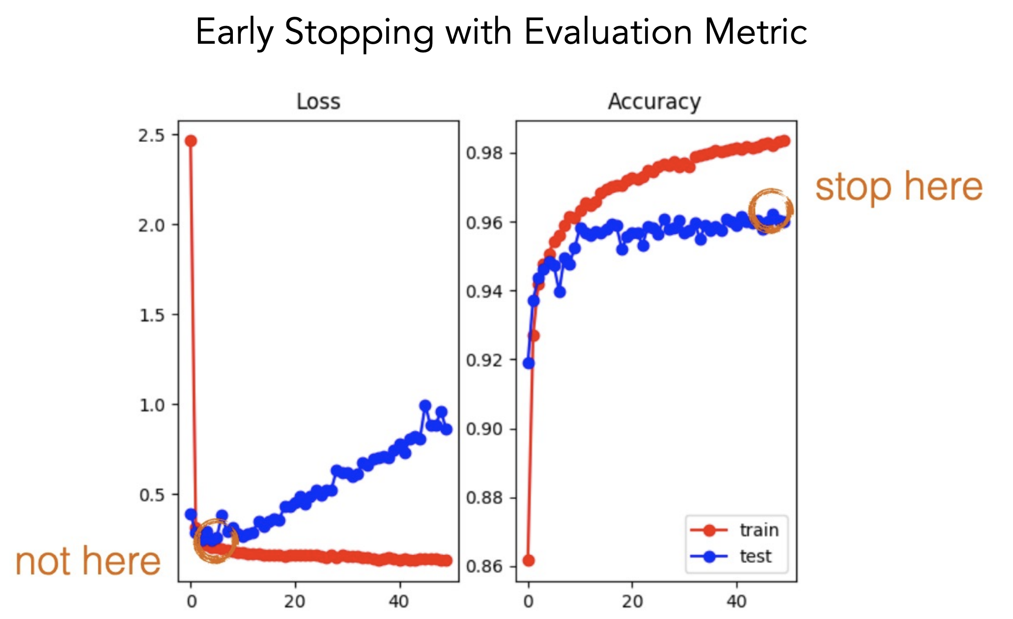
Early Stopping
Early stop on the evaluation metric not the loss b/c the two aren’t necessarily correlated
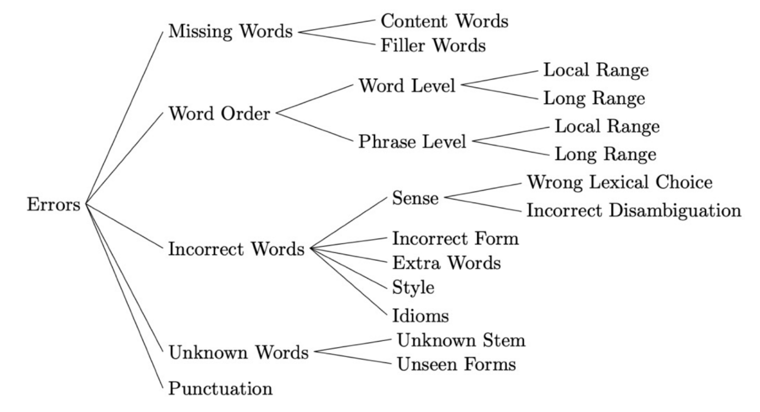
Common NLP Types of Errors
Interpretable Methods
- LIME
- Attention
Tools
- BERTology - access all hidden states of BERT
- AllenNLP Interpret
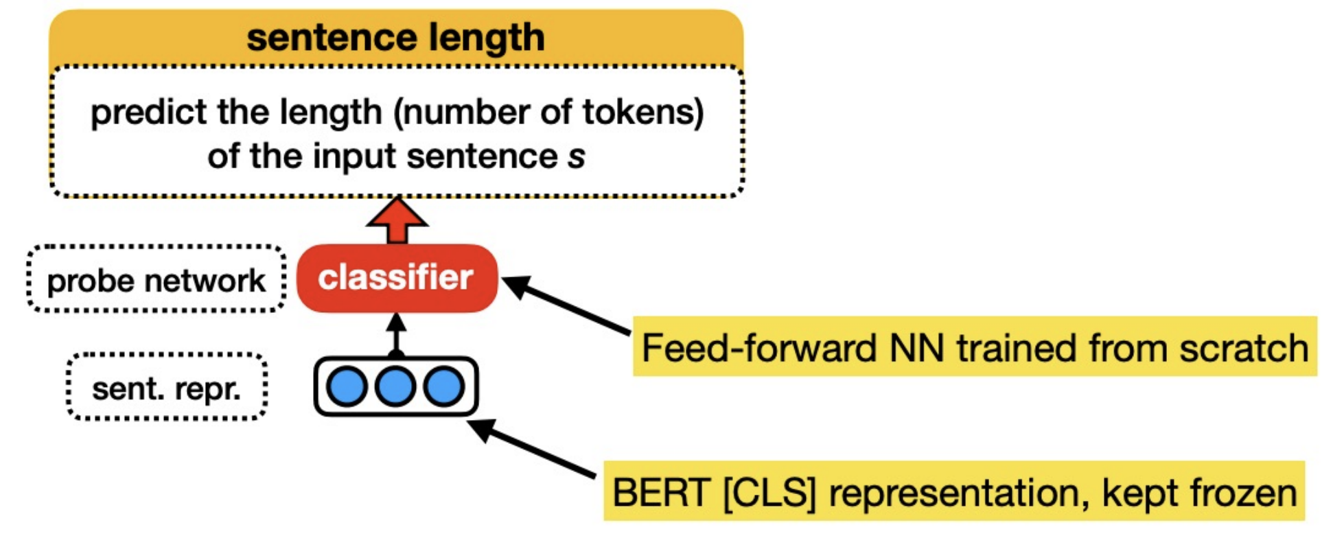
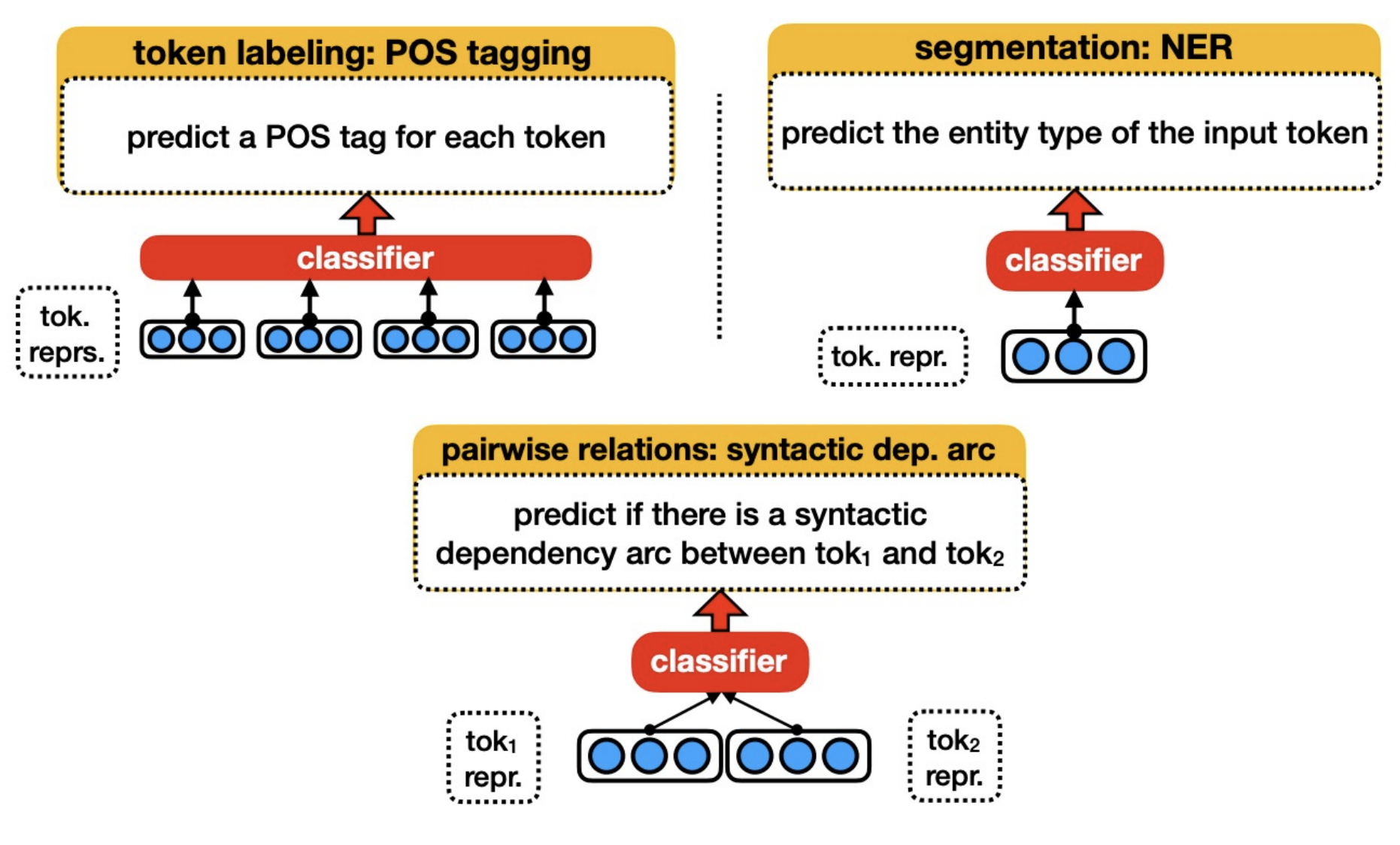
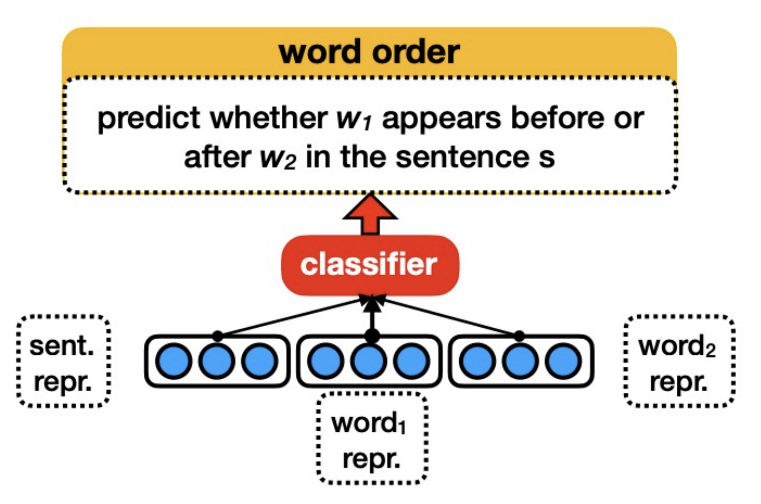
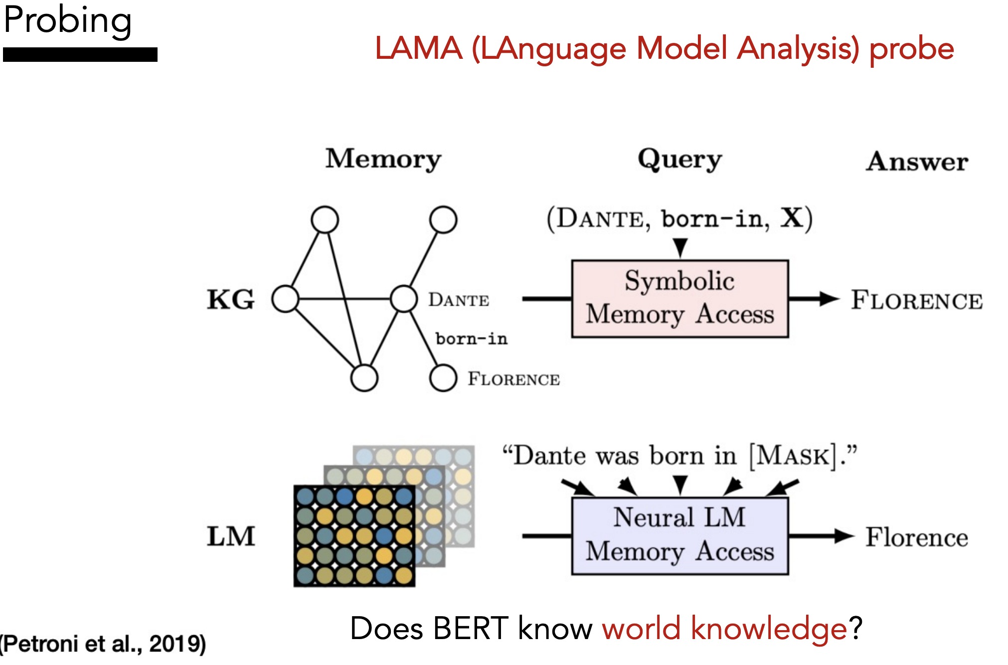
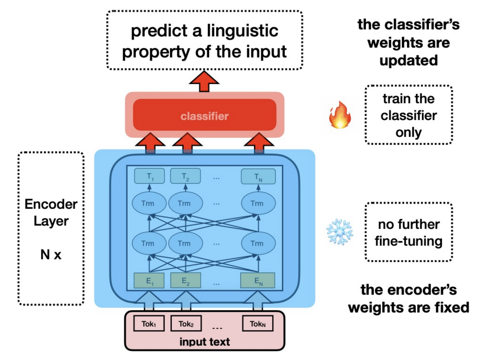
Probing
Goal: Understand + interpret the language features that the model is encoding in its embeddings
Idea: Fix BERT, extract an input’s representation, feed that representation into a classifier to predict some linguistic property of the input, if the classifier is able to predict it then that property must be encoded somewhere in the representation.
Want “high selectivity” (Hewitt et al. 2019)
Examples: