Let’s say we have a transformer model taken from HuggingFace.

How do we determine…

1. It’s parameter count?
2. It’s memory requirement?
3. It’s network architecture?

In Part 1 of this 3-Part series, we’ll use GPT2 as an illustrative example and walk through each step. We’ll explain how to calculate the parameter count of a transformer model, how to calculate its training and inference memory requirements, and how to visualize its underlying architecture.

The lessons should generalize to any PyTorch model.

For this Part 1, we will focus on answering the question:

How many parameters does GPT2 have?

Parameter Count

We begin by loading GPT2.

!pip install transformers torch

from transformers import GPT2Model
model = GPT2Model.from_pretrained('gpt2')

Let’s print out the layers of the model, and define a helper function for counting each layer’s parameters.

def count_params(model, is_human: bool = False):
    params: int = sum(p.numel() for p in model.parameters() if p.requires_grad)
    return f"{params / 1e6:.2f}M" if is_human else params

print(model)
print("Total # of params:", count_params(model, is_human=True))

GPT2Model(
  (wte): Embedding(50257, 768)
  (wpe): Embedding(1024, 768)
  (drop): Dropout(p=0.1, inplace=False)
  (h): ModuleList(
    (0-11): 12 x GPT2Block(
      (ln_1): LayerNorm((768,), eps=1e-05, elementwise_affine=True)
      (attn): GPT2Attention(
        (c_attn): Conv1D()
        (c_proj): Conv1D()
        (attn_dropout): Dropout(p=0.1, inplace=False)
        (resid_dropout): Dropout(p=0.1, inplace=False)
      )
      (ln_2): LayerNorm((768,), eps=1e-05, elementwise_affine=True)
      (mlp): GPT2MLP(
        (c_fc): Conv1D()
        (c_proj): Conv1D()
        (act): NewGELUActivation()
        (dropout): Dropout(p=0.1, inplace=False)
      )
    )
  )
  (ln_f): LayerNorm((768,), eps=1e-05, elementwise_affine=True)
)
Total # of params: 124.44M

So GPT2 contains a total of 124.44M trainable parameters.

OK, that was easy.

What does this actually mean?

Let’s break it down layer by layer, then come up with an overall formula for the parameter count of GPT2.

Layer-by-Layer Parameter Count

First, let’s define a few constants.

• V = number of tokens in our vocabulary. (For GPT2, this is $50257$)
• E = the size of the embedding vector. (For GPT2, this is $768$)
• P = the maximum sequence length that our model can handle. (For GPT2, this is $1024$).

Embedding Layers

Let’s start by analyzing the first two layers in our GPT2 model, wte and wpe.

wte

• This is an Embedding layer.
• This is responsible for embedding our input tokens.
• It is a matrix of size V (50257) by E (768).
• In other words, our vocabulary has a total of 50257 unique tokens, and each token is represented by a dense vector of 768 floating point numbers.

Params = $V * E = 50257 * 768 = 38,603,776$

wpe

• This is an Embedding layer.
• This is responsible for embedding the positions of our input tokens.
• It is a matrix of size P (1024) by E (768).
• This means that the maximum sequence length that our model can handle is 1024 tokens. This is also referred to as the “context window.”
• Just like the tokens themselves, each position is represented by a dense vector of 768 floating point numbers.

Params = $P * E = 1024 * 768 = 786,432$

The embeddings from these two layers will get added together to create “position-aware” embeddings of our input tokens.

Let’s verify our math with some code:

V: int = model.config.vocab_size
E: int = model.config.n_embd
P: int = model.config.n_positions
expected_wte = V * E
expected_wpe: int = P * E
print(f"wte | Expected: {expected_wte}")
print(f"wte | True:     {count_params(model._modules['wte'])}")
print(f"wpe | Expected: {expected_wpe}")
print(f"wpe | True:     {count_params(model._modules['wpe'])}")

wte | Expected: 38597376
wte | True:     38597376
wpe | Expected: 786432
wpe | True:     786432

Transformer Layers

Now, let’s move onto the exciting part: the actual transformer layers.

These are marked as h in the printout above. (We’ll skip the drop layers for now.)

Each transformer layer is called GPT2Block. By the (0-11) 12 x GPT2Block notation, we can see that there are 12 transformer layers in total. Each layer is identical – we just stack them on top of each other 12 times in a row, hence the 12 x notation. We’ll just analyze one of them, then multiply by 12 to get the total.

Let’s breakdown the components of a transformer layer.

ln_1

• This is a LayerNorm layer.
• This is responsible for “normalizing” the input before it is passed to the attention layer. It normalizes across the last dimension, which is the embedding dimension. This means that the values along the embedding dimension will be normally distributed with a mean of 0 and a standard deviation of 1.
• The eps=1e-5 parameter is the value $\epsilon$ added to the denominator. It is used for numerical stability, to prevent division by zero.
• The elementwise_affine=True parameter means that the layer will learn a bias $\beta$ and gain $\gamma$ for each embedding dimension.
• The formula for LayerNorm is as follows:

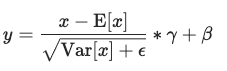
• $E[x]$ and $Var[x]$ are calculated on the fly as the mean of the input ($x$) across the embedding dimension.
• Thus, the only learnable parameters here are $\beta$ and $\gamma$, which are vectors of size E (768).

Params = $2 * E = 2 * 768 = 1536$

Let’s verify our math with some code:

expected_ln_1 = 2 * E
print(f"ln_1 | Expected: {expected_ln_1}")
print(f"ln_1 | True:     {count_params(model._modules['h'][0].ln_1)}")

ln_1 | Expected: 1536
ln_1 | True:     1536

attn

• This is a GPT2Attention layer, aka “self-attention”.
• This computes the self-attention scores between each token in the input sequence.
• It is comprised of four sub-layers:
  • c_attn
    • This is a Conv1D layer.
    • This confused me for a while. What was this Conv1D layer doing in the middle of a transformer layer? I thought it was supposed to be an MLP? My understanding is that it is basically a linear layer, but with the weights transposed. I’m not sure what motivated this design decision, so if anyone knows please leave a comment.
    • It is responsible for transforming the input into the query, key, and value matrices for the attention calculation.
    • It is a matrix of size E (768) by 3 * E (2304) plus a bias vector of size 3 * E (2304). The 3 * E is because we have 3 inputs to the attention layer: the query, the key, and the value. Each of these inputs is a vector of size E (768), so we have to generate a total of 3 * E (2304) elements.
  • c_proj
    • This is a Conv1D layer.
    • It is responsible for combining the outputs of the attention heads (in our case, there are $12$ heads amongst which $768$ dims are equally divided, which gives each head a $64$-dim output).
    • It is a matrix of size E (768) by E (768) plus a bias vector of size E (768).
  • attn_dropout
    • This is a Dropout layer.
    • It is responsible for dropping out a fraction ($p = 0.1$) of activations post-attention calculation during training.
    • This has no trainable parameters.
  • resid_dropout is a Dropout layer.
    • It is responsible for dropping out a fraction ($p = 0.1$) of activations post-projection during training.
    • This has no trainable parameters.

Params = c_attn + c_proj + attn_dropout + resid_dropout = $[E * (3 * E) + (3 * E)]$ + $[E * E + E]$ + $0$ + $0$ = $4 E^2$ + $4E$ = $4 * 768^2 + 4 * 768 = 2,362,368$

Let’s check our work:

expected_c_attn = E * (3 * E) + (3 * E)
expected_c_proj = E * E + E
expected_attn_dropout = 0
expected_resid_dropout = 0
expected_attn = expected_c_attn + expected_c_proj + expected_attn_dropout + expected_resid_dropout
print(f"c_attn | Expected: {expected_c_attn}")
print(f"c_attn | True:     {count_params(model._modules['h'][0].attn.c_attn)}")
print(f"c_proj | Expected: {expected_c_proj}")
print(f"c_proj | True:     {count_params(model._modules['h'][0].attn.c_proj)}")
print(f"attn_dropout | Expected: {expected_attn_dropout}")
print(f"attn_dropout | True:     {count_params(model._modules['h'][0].attn.attn_dropout)}")
print(f"resid_dropout | Expected: {expected_resid_dropout}")
print(f"resid_dropout | True:     {count_params(model._modules['h'][0].attn.resid_dropout)}")
print(f"attn | Expected: {expected_attn}")
print(f"attn | True:     {count_params(model._modules['h'][0].attn)}")

c_attn | Expected: 1771776
c_attn | True:     1771776
c_proj | Expected: 590592
c_proj | True:     590592
attn_dropout | Expected: 0
attn_dropout | True:     0
resid_dropout | Expected: 0
resid_dropout | True:     0
attn | Expected: 2362368
attn | True:     2362368

ln_2

• This is another LayerNorm layer.
• It is basically the same thing as ln_1 described above.

Params = $2 * E = 2 * 768 = 1536$

Let’s check our work again:

expected_ln_2 = 2 * E
print(f"ln_2 | Expected: {expected_ln_2}")
print(f"ln_2 | True:     {count_params(model._modules['h'][0].ln_2)}")

ln_2 | Expected: 1536
ln_2 | True:     1536

Let’s now define one more constant:

• H = the size of the hidden layer within each transformer layer. (For GPT2, this is $3072$)

mlp

• This is a GPT2MLP layer, aka the “feed-forward layer” or “multi-layer perceptron”.
• This is responsible for providing most of the “computational oomph” of the transformer. It is applied to each token separately.
• It is comprised of four sub-layers:
  • c_fc
    • This is a Conv1D layer.
    • Again, you can simply think of this as a linear layer.
    • It is responsible for “up-projecting” the output of the attention layer into a hidden space of dimension H. You will often see H = 4 * E. Why 4 * E? I think this is simply by convention. The original paper uses H = 4 * E, and it seems like most implementations follow suit. You want this to be big enough to give the model enough expressivity to model complex functions, but not so big that it becomes computationally intractable.
    • It is a matrix of size E (768) by H (3072), with a bias vector of size H (3072).
  • c_proj
    • This is a Conv1D layer.
    • Again, this is basically a linear layer.
    • It is responsible for “down-projecting” the output of the first feed-forward layer c_fc back into the embedding space. This allows us to immediately pass its output into the next transformer layer (which, as you may recall, expects an input of size E (768) in ln_1).
    • It is a matrix of size H (3072) by E (768), with a bias vector of size E (768).
  • act
    • This is a NewGELUActivation layer.
    • It is responsible for applying the GELU activation function to the output of c_fc.
  • dropout
    • This is a Dropout layer.
    • It is responsible for dropping out a fraction ($p = 0.1$) of activations post-down-projection.
    • This has no trainable parameters.

Params = c_fc + c_proj + act + dropout = $[E * H + H]$ + $[H * E + E]$ + $0$ + $0$ = $2 E H + E + H$ = $8 * 768^2 + 768 + 3072$ = $4,722,432$

Let’s check our work again:

H: int = 4 * E
expected_c_fc = E * H + H
expected_c_proj = H * E + E
expected_act = 0
expected_dropout = 0
expected_mlp = expected_c_fc + expected_c_proj + expected_act + expected_dropout
print(f"c_fc | Expected: {expected_c_fc}")
print(f"c_fc | True:     {count_params(model._modules['h'][0].mlp.c_fc)}")
print(f"c_proj | Expected: {expected_c_proj}")
print(f"c_proj | True:     {count_params(model._modules['h'][0].mlp.c_proj)}")
print(f"act | Expected: {expected_act}")
print(f"act | True:     {count_params(model._modules['h'][0].mlp.act)}")
print(f"dropout | Expected: {expected_dropout}")
print(f"dropout | True:     {count_params(model._modules['h'][0].mlp.dropout)}")
print(f"mlp | Expected: {expected_mlp}")
print(f"mlp | True:     {count_params(model._modules['h'][0].mlp)}")

c_fc | Expected: 2362368
c_fc | True:     2362368
c_proj | Expected: 2360064
c_proj | True:     2360064
act | Expected: 0
act | True:     0
dropout | Expected: 0
dropout | True:     0
mlp | Expected: 4722432
mlp | True:     4722432

Other Layers

Our last layer is one final Layer Norm.

ln_f

• This is another LayerNorm layer.
• It is basically the same thing as ln_1 described above.

Params = $2 * E = 2 * 768 = 1536$

Let’s check our work again:

expected_ln_f = 2 * E
print(f"ln_f | Expected: {expected_ln_f}")
print(f"ln_f | True:     {count_params(model._modules['ln_f'])}")

ln_f | Expected: 1536
ln_f | True:     1536

Overall Formula for GPT2 Parameter Count

Putting everything together, we get the following formula for the parameter count $C$ of GPT2:

where

• V = number of tokens in our vocabulary. (For GPT2, this is $50257$)
• E = the size of the embedding vector. (For GPT2, this is $768$)
• P = the maximum sequence length that our model can handle. (For GPT2, this is $1024$).
• L = the number of transformer layers. (For GPT2, this is $12$)
• H = the size of the hidden layer within each transformer layer. (For GPT2, this is $3072$)

Plugging in our numbers, we get:

Let’s check our work one final time:

L: int = model.config.n_layer
expected_gpt2: int = E * (V + P) + L * (12 * E * E + 13 * E) + (2 * E)
print(f"gpt2 | Expected: {expected_gpt2}")
print(f"gpt2 | True:     {count_params(model)}")

gpt2 | Expected: 124439808
gpt2 | True:     124439808

Woohoo! We’ve successfully counted every parameter of GPT2.

It turns out that GPT2 has 124.44M trainable parameters.

Conclusion

You can basically repeat this process for any PyTorch model to get its parameter count.

Stay tuned for Part 2 in which we calculate the memory requirements of training and running inference with GPT2.

References

• Illustrated Transformer
• Annotated Transformer
• Transformer Math