Motivating Question: How do diffusion models work?

Goals:

1. Understand the high-level intuition of diffusion models
2. Derive the math behind diffusion models
3. Implement a diffusion model from scratch in Python

In this post, we’ll explore the basics of diffusion models and try to implement them from scratch in Python.

Important Disclaimer: I am not an expert by any means – this is my attempt to teach myself diffusion models, so parts of this are probably inaccurate. If you find any errors, please let me know!

Table of Contents

1. High-Level Intuition (without Math)
2. High-Level Intuition (with Math)
3. Mathematical Derivation
4. Code (with Math)

High-Level Intuition (without Math)

In this section, I provide super basic intuition without any math. If you’re already familiar with diffusion models, feel free to skip to the next section.

What is a diffusion model?

A “diffusion model” is a generative model that learns how to add random noise to data and remove random noise from data.

The “add random noise to data” part is called the “forward process,” while the “remove random noise from data” is the “reverse process.”

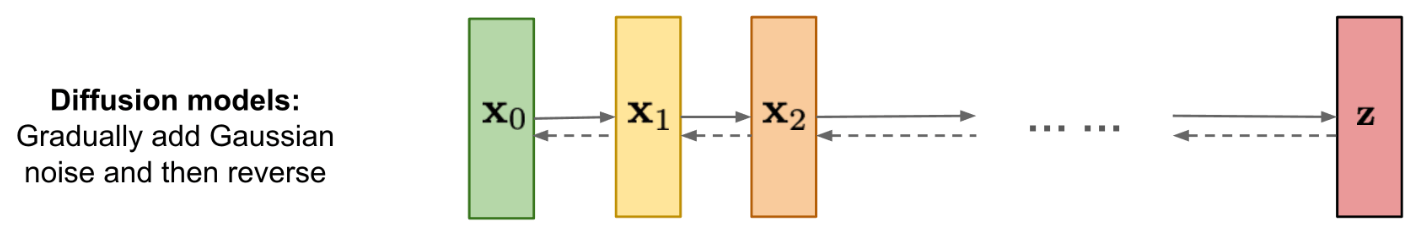Picture Credit: https://lilianweng.github.io/posts/2021-07-11-diffusion-models/

Diffusion models are useful because they can generate virtually infinite amounts of realistic data from scratch.

A popular application is image generation, in which you tell the diffusion model what you want in English and it generates a completely novel image.

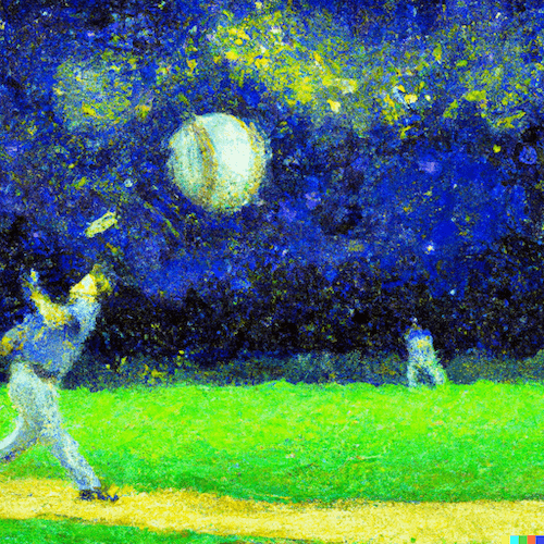
Prompt to DALL-E: “an impressionist painting in the style of van gogh starry night of a baseball being thrown”

Popular diffusion models include DALL-E, MidJourney, and Stable Diffusion.

Forward v. Reverse Process

Clearly, one of these processes is much harder than the other – it’s much easier to add random noise to data than it is to recover the original data from a noisy version of it.

That’s because the forward process doesn’t actually require learning anything – the model is just adding random noise to data.

The reverse process of recovering data from noise is much harder. This is the task that diffusion models are trying to learn.

Here’s an analogy to make this distinction between “forward” and “reverse” clearer:

Let’s say I gave you a Jackson Pollock painting and told you to “add noise to it” i.e. do the “forward process.”

To “add noise,” you might take a bucket of paint and throw it at the painting. This is pretty easy for you to do.

Now let’s say I find a different Jackson Pollock painting, and I throw a bucket of paint on it.

Your new task is to remove all the paint that I threw onto the painting i.e. do the “reverse process” of recovering the original “data” (i.e. painting) from the “noised version” of it (i.e. the painting with extra random paint added to it).

This is clearly a much harder task.

You would probably have to spend a lot of time and effort to remove all the paint (“random noise”) I added. You wouldn’t know which pieces of paint were part of the original painting and which paint was added by me, so while you could probably get pretty close to the original painting depending on how much “noise” (i.e. paint) I added, you probably would never be able to recover the original painting perfectly.

Because learning the reverse process is hard, we purposely design the forward process to make reversing it easy.

We do this in two ways:

1. We split the forward process into many small steps.
2. We only add a small amount of noise to the data at each step of the forward process.
3. The random noise we add is Gaussian noise.

Why do we care about the reverse process?

What’s the point of learning the seemingly arbitrary task of removing noise from data?

Well, once the model learns how to run the “reverse process,” it can then be used to generate new data from scratch. The reverse process is the key to unlocking our model’s generative ability.

Here’s how that works:

1. We give the model random noise (which we can easily generate ourselves)
2. We ask the model to remove the noise and recover the original data.
3. Here’s the trick: there was no actual “original data” to begin with. But the model doesn’t know that. It thinks that the random noise we gave it was added to some original data, and it will try its best to recover that original data.
4. The model will output its guess as to what data could have led to that noised version of itself. If we’ve trained the model well, then when it tries to recover the original data, it will actually generate new data that looks like the original data we trained it on.

As long as we can generate arbitrary configurations of random noise, then the model will keep generating outputs that look like our original dataset (but are hopefully different). Thus, we can generate infinite realistic data.

How do we teach the model the reverse process (i.e. “training”)?

At a high level, the training process works as follows: we take a dataset of real data, sample a random example from the dataset, and add random noise to it. Then, we feed the noised version of the sampled example into our diffusion model, and have it predict the noise that was added to the image. Finally, we update the model’s parameters to make it more likely that the model will predict the correct noise in the future.

To make this section more concrete, let’s say that we’re specifically training a diffusion model to generate images of human faces.

Our goal is to have the model learn how to go from random noise -> realistic human faces.

Thus, our “forward process” will be adding random noise to images of human faces, and the “reverse process” will be generating human faces from random noise.

To train the model, we’ll first collect a dataset of images of real human faces.

Next, we follow the steps below to train it:

1. Sample a random image from our dataset of human faces.
2. Forward process: Add random noise to the image to generate a noised image.
3. Reverse process: Feed the noised image into our machine learning model, and have it predict the noise in the image.
4. Compare the predicted noise to the actual noise we added in step 2.
5. Update the model’s parameters to make it more likely to predict the correct noise in the future.
6. Repeat steps 1-5 until the model is good at predicting the noise in a noised image.

Once the model is good at predicting the noise in a noised image, we can then use it to generate new images of human faces.

How do we use the model to generate new examples (i.e. “inference”)?

Continuing our example of the human face diffusion model, the procedure of generating new data (also referred to as “inference” or “denoising”) would work as follows:

1. Generate an image of random noise.
2. Feed the random noise into our trained model, and have it predict the noise in the image.
3. Subtract the predicted noise from the random noise to get a slightly less noisy version of the image.
4. Repeat steps 1-3 until the model outputs an image that looks like a human face.

High-Level Intuition (with Math)

In this section, we’ll add some math to our intuition. This requires some basic knowledge of probability and statistics, but I’ll try to explain everything as clearly as possible.

What is a diffusion model?

A “diffusion model” is a generative model which learns to reverse a Markov process in which noise is incrementally added to the data.

The forward process adds noise to the data, while the reverse process removes noise from the data.

Assume we are given a dataset $D = {x^{(1)}, x^{(2)}, …, x^{(n)}}$ containing $n$ examples of data. For the sake of simplicity, let’s focus on a specific datapoint $\mathbf{x}$ for the remainder of this section. We’ll refer to the underlying data distribution from which $D$ is generated as $q(\mathbf{x})$.

The forward process occurs over a series of timesteps $t = 0, 1, 2, …, T$. As $t$ increases, more and more noise is added to our datapoint $\mathbf{x}$. We’ll refer to our datapoint at timestep $t$ as $\mathbf{x}_t$.

Let $\mathbf{x}_0 \sim q(\mathbf{x})$ be a datapoint sampled from our data distribution without any sort of modifications.

Then $\mathbf{x}_T$ is the final noised version of that datapoint after $T$ steps of our forward process have been applied to $\mathbf{x}_0$.

We will now define precisely what we mean by “forward” and “reverse” process.

Forward Process

The forward process is a Markov chain that incrementally adds noise to our data, i.e. given $\mathbf{x}_{t-1}$ it generates $\mathbf{x}_t$ by adding noise to $\mathbf{x}_{t-1}$.

The fact that we’ve defined this forward process to be Markovian means that the probability of transitioning from one state $t-1$ to state $t$ depends only on state $t-1$, and not on any previous states.

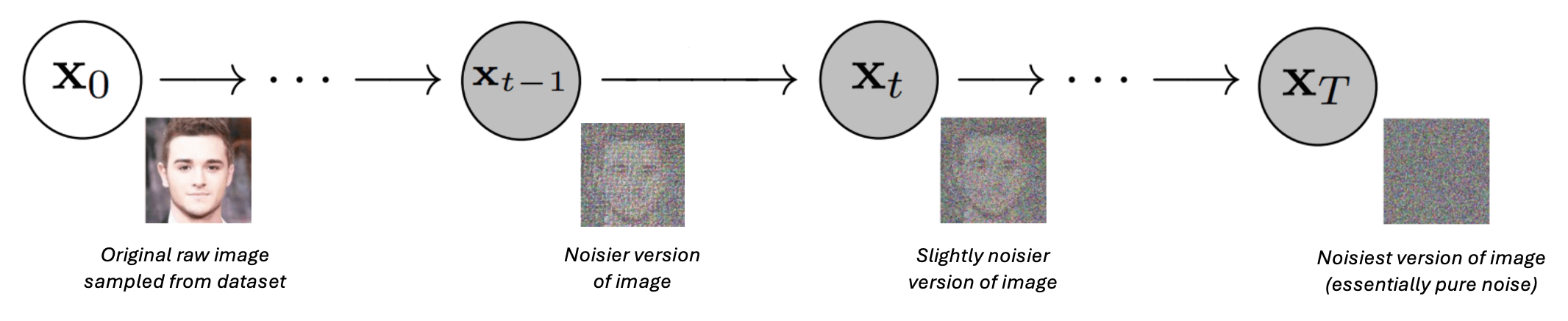Forward process. Credit: AssemblyAI

Formally, we define the probability of transitioning from state $\mathbf{x}_{t-1}$ to state $\mathbf{x}_t$ as $q(\mathbf{x}_t \vert \mathbf{x}_{t-1})$ for all $t \in {1, …, T}$.

Note that by the definition of a Markov process, we have that $q(\mathbf{x}_t \vert \mathbf{x}_{t-1}) = q(\mathbf{x}_t \vert \mathbf{x}_T, …, \mathbf{x}_{t-1}, \mathbf{x}_{t-2}, …, \mathbf{x}_0)$ since $\mathbf{x}_t$ is conditionally independent of all other states given $\mathbf{x}_{t-1}$.

This also means that:

Which can be seen in the following diagram:

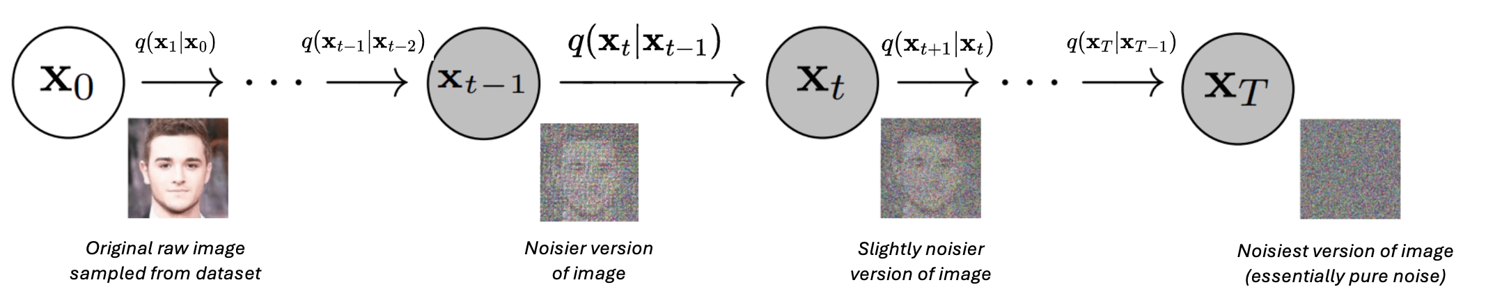Forward process with $q$ annotated. Credit: AssembyAI

Reverse Process

The reverse process is a Markov chain that incrementally removes noise from the data, i.e. given $\mathbf{x}_t$ it generates $\mathbf{x}_{t-1}$ by removing noise from $\mathbf{x}_t$.

The reverse process is shown below. Note that this is simply the opposite of the forward process depicted above.

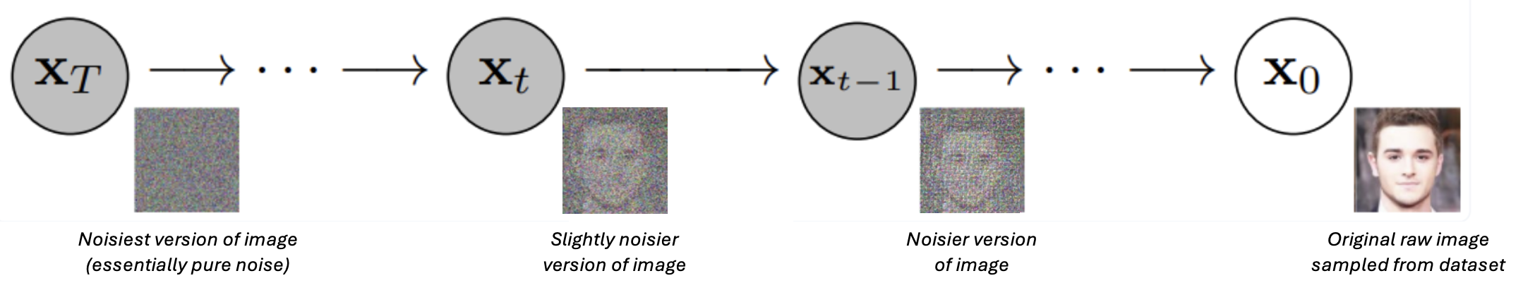Reverse process. Credit: https://www.assemblyai.com/blog/diffusion-models-for-machine-learning-introduction/

The reverse process is defined via a probability distribution $p(\mathbf{x}_t \vert \mathbf{x}_{t-1})$ which represents the probability of transitioning from state $\mathbf{x}_t$ to state $\mathbf{x}_{t-1}$.

Since the reverse process is Markovian, we have that:

Why can we make this assumption that the reverse process is a Markov chain (just like the forward process)? My understanding is this property comes from the fact that the noise we add at each step of the forward process is sufficiently small.

Our goal is to learn $p$, i.e. the probability distribution that parametrizes the reverse process.

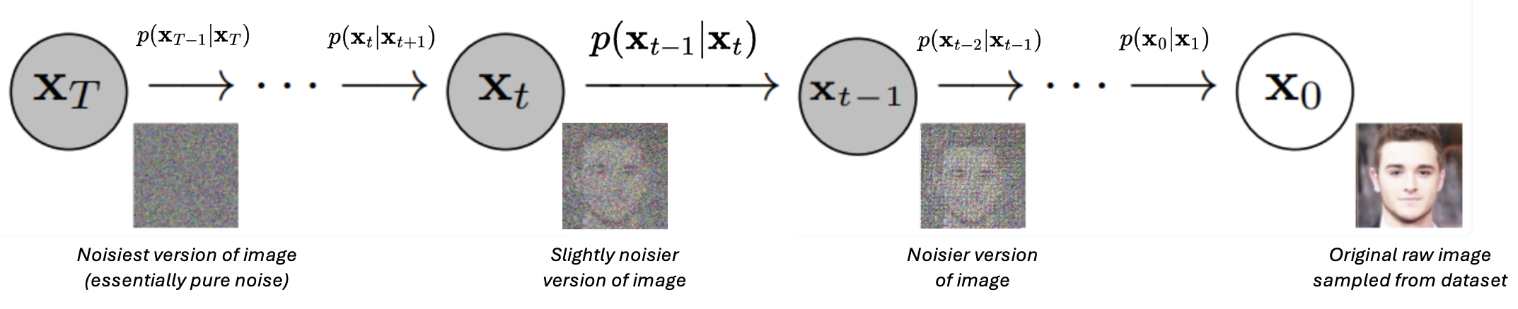Reverse process with $p$ annotated. Credit: AssemblyAI

Forward v. Reverse Process

This diagram does a good job of showing how the forward and reverse processes are related:

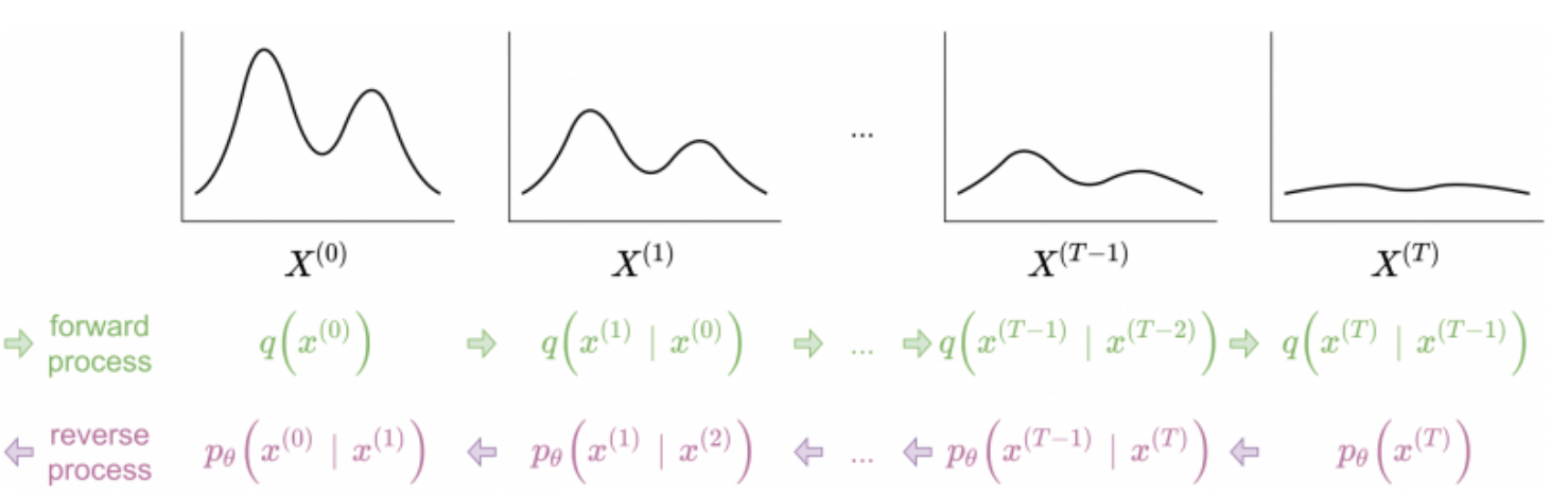Credit: https://deeprender.ai/blog/discrete-denoising-diffusion-models

How do we teach the model the reverse process (i.e. “training”)?

To train our model, we will (roughly) follow the following steps:

1. Sample a random datapoint $\mathbf{x}_0 \sim q(\mathbf{x})$ from our dataset.
2. Sample a time step $t’ \sim \text{Uniform}(1, …, T)$.
3. Sample a noise vector $\mathbf{\epsilon} \sim \mathcal{N}(0, \mathbf{I})$.
4. Run the forward process on $\mathbf{x}_0$ by repeatedly applying $q(\mathbf{x}_t \vert \mathbf{x}_{t-1})$ for $t = { 1, …, t’ }$ to generate $\mathbf{x}_{t’}$.
5. Given $t’$ and $\mathbf{x}_{t’}$, have the model predict the noise vector $\mathbf{\epsilon}$ that was added to $\mathbf{x}_0$.
6. Calculate the loss (i.e. squared error) between the predicted and true noise vectors.
7. Update the model’s parameters using gradient descent on the loss.

By the end of the training process, our model will have effectively learned $p(\mathbf{x}_t \vert \mathbf{x}_{t-1})$.

How do we use the model to generate new examples (i.e. “inference”)?

To generate new data, we will (roughly) follow the following steps:

1. Sample an image of completely random noise $\mathbf{x}_T \sim \mathcal{N}(0, \mathbf{I})$.
2. Incrementally remove noise from $\mathbf{x}_T$ by repeatedly applying $p(\mathbf{x}_t \vert \mathbf{x}_{t-1})$ for $t = T, …, 0$.
3. Return the generated $\mathbf{x}_0$.

Comparison to other generative ML models

Here is how diffusion models compare to other generative models common in machine learning:

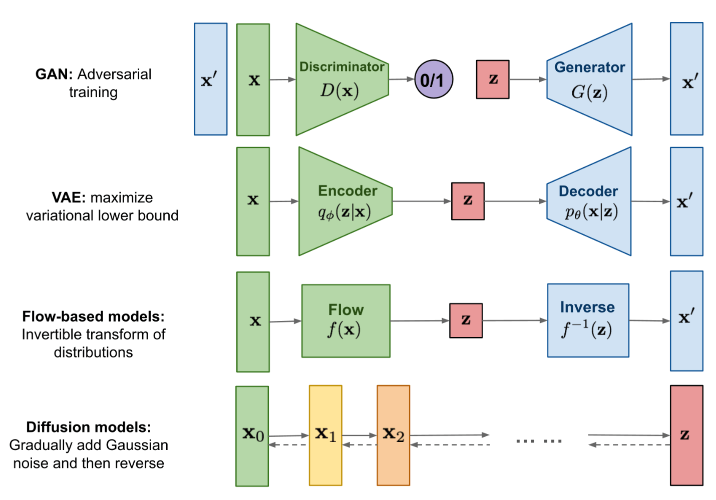Credit: https://lilianweng.github.io/posts/2021-07-11-diffusion-models/

Mathematical Derivation

In this section, I will do my best to walk through the math behind diffusion models, as originally detailed in the denoising diffusion probabilistic models (DDPM) paper (Ho et al., 2020).

This is a diffusion model that adds/removes Gaussian noise to continuous data, e.g. images.

Forward Process

We start by sampling a real data point $\mathbf{x}_0$ from our dataset $D$. This is written notationally as:

Remember that we defined our forward process $q(\mathbf{x}_1, \dots, \mathbf{x}_T \vert \mathbf{x}_{0})$ as a Markov chain. Thus, we can rewrite the joint probability of the entire noising process from $t = 0$ to $t = T$ for our sampled real data point $\mathbf{x}_0$ as the following:

Let us assume that we add a small amount of Gaussian noise to our datapoint at each step of our forward process. This is written notationally as:

Which can also be expressed as:

Let’s make this concrete. Say that $\mathbf{x}_{t-1}$ is an image where an individual pixel $i$ is denoted as $x^{i}_{t-1}$ (note: this is now a scalar rather than a vector since we’re looking at an individual element, i.e. pixel, of $\mathbf{x}_{t-1}$). Then the above equation is saying that $x^{i}_t$ is sampled from a Normal distribution centered at $x^{i}_{t-1}$ with a standard deviation of 1.

What if we want our noise to have a standard deviation other than 1?

We can simply multiply the standard deviation by an adjustable parameter $\beta$. We sometimes want $\beta$ to depend on the time step $t$, so we specificallyrewrite this as $\beta_t$. We now have a “variance schedule” of $\beta_1, \dots, \beta_T$, which gives us:

There is one lingering issue with this equation: the variance will increase with each step that we move through the forward process. This is referred to as “exploding variance,” and will make it harder for our model to learn the reverse process.

To see this issue of “exploding variance,” let’s explicitly calculate the variance of $\mathbf{x}_t$.

First, let’s write out the definition of $\mathbf{x}_{t}$ given $\mathbf{x}_{t-1}$ and $\mathbf{\epsilon}_{t-1} \sim \mathcal{N}(0, \mathbf{I})$.

Remembering that two independent Gaussians $A = \mathcal{N}(\mu_A, \sigma_A^2)$ and $B = \mathcal{N}(\mu_B, \sigma_B^2)$ can be added together to form a new Gaussian $C = A + B = \mathcal{N}(\mu_A + \mu_B, \sigma_A^2 + \sigma_B^2)$, we have that:

Where Step (4) is because $\mathbf{\epsilon}_{t-2}$ and $\mathbf{\epsilon}_{t-1}$ are independent standard Normals, thus we can add them together as $\mathbf{\epsilon} \sim N(0, \mathbf{I})$.

For independent variables $A,B$ and a constant $c$, remember that $VAR(cA + B) = c^2 VAR(A) + VAR(B)$. Thus, the variance of $\mathbf{x}_t$ is given by:

Thus, with each successive $t$, our variance $\mathbf{x}_t$ increases by $\beta_t$. This is not ideal, since it will make it harder for our model to learn the reverse process.

Ideally, we want to better control the variance of $\mathbf{x}_t$ as $t$ increases. To accomplish this, we will add a scaling factor to our mean of $\sqrt{1 - \beta_t}$.

To be completely honest, I don’t fully understand where the expression $\sqrt{1 - \beta_t}$ is derived from. If you have any insight, please leave a comment!

Thus, our final expression for the forward process is:

If we want to calculate $\mathbf{x}_T$, we can simply apply the above equation $T$ times, starting with $\mathbf{x}_0$.

However, this is computationally inefficient.

Instead, we can use a shortcut that simply requires conditioning on $\mathbf{x}_0$.

Let’s start by defining a few helpful expressions:

Next, let’s write out the formula for $\mathbf{x}_t$ again, but this time in terms of $\alpha_t$ and $\bar{\alpha}_t$:

And now let’s simply things down to $\mathbf{x}_0$:

Great! We now have a way of jumping directly from $\mathbf{x}_0$ to $\mathbf{x}_t$, without having to apply the forward process $t$ times.

Thus, we have that:

Reverse Process

TBD

Code (with Math)

In this section, we’ll implement a diffusion model from scratch in Python.

I will interleave the math with the code so that you can see how it all connects.

Setup

First, let’s import a bunch of libraries and load our dataset of images that we can add / remove noise from.

!pip install numpy torch torchvision matplotlib jaxtyping ipykernel

import time
import random
import argparse
import torch
import torchvision
import numpy as np
import matplotlib.pyplot as plt
from typing import List
from jaxtyping import Float
from tqdm import tqdm

random.seed(1)

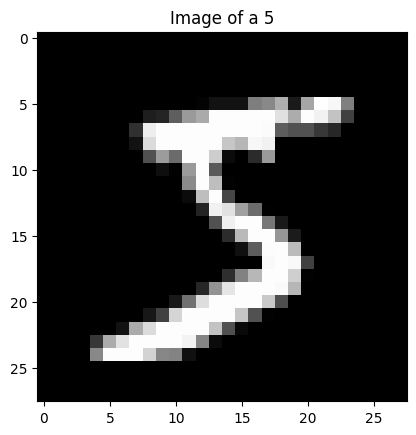
For our dataset we’ll use MNIST, which contains images of handwritten digits.

Each image is grayscale and has dimensions 28x28 pixels.

# First, let's get the MNIST dataset
## This `transform` does two things: (1) converts the image to a PyTorch tensor, and (2) normalizes the image to have pixel values between [-1, 1]
transform = torchvision.transforms.Compose([
    torchvision.transforms.ToTensor(), 
    torchvision.transforms.Normalize((0.5,), (0.5,))
])
## Download the `train` split of the MNIST dataset, then apply our `transform` to each image
train_dataset = torchvision.datasets.MNIST('~/.pytorch/MNIST_data/', 
                                           download=True, 
                                           train=True, 
                                           transform=transform)
## Create a `DataLoader` object so that we can load our MNIST dataset in batches
train_dataloader = torch.utils.data.DataLoader(train_dataset, batch_size=16, shuffle=False)

Let’s view an example image from our dataset.

A couple things to note about the raw numerical representation of each image:

1. The image is represented as a 3D array of floating point numbers, where each number represents the intensity of a pixel in the image.
   1. The 1st dimension represents the channels of the image. Since this is a grayscale image, we only have one channel. If this were a color image, we would have three channels (one for each color: red, green, and blue).
   2. The 2nd dimension is the height of the image.
   3. The 3rd dimension is the width of the image.
2. All of the pixels have been scaled to have a value between [-1, 1] per our transformation step above.

# As a sanity check, let's view a random image from our dataset
C: int = 1 # number of channels
W: int = 28 # width of image (pixels)
H: int = 28 # height of image (pixels)
image: Float[torch.Tensor, "1 28 28"] = train_dataset[0][0]
label: int = train_dataset[0][1]

print(f"Label: {label} | Channels: {image.shape[0]} | Height: {image.shape[1]}px | Width: {image.shape[2]}px")
plt.imshow(image[0,:,:], cmap='gray') # remove first dimension (channels)
plt.title(f'Image of a {label}')
plt.show()

Label: 5 | Channels: 1 | Height: 28px | Width: 28px

Forward Process

Now that we have our dataset, let’s implement the forward process.

First, let’s define the variables we’ll need for the forward process:

T: int = 50 # number of total steps
betas: Float[np.ndarray, "T"] = torch.linspace(1e-4, 1e-1, T) # beta_t's
alphas: Float[np.ndarray, "T"] = 1 - betas # alpha_t's
alpha_bars: Float[torch.Tensor, "T"] = torch.Tensor(np.cumprod(alphas)) # alpha_bar_t's
sigmas: Float[torch.Tensor, "T"] = torch.sqrt(betas) # sigma_t's

Now let’s run the forward process itself.

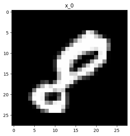
First, sample a random image from our dataset:

random.seed(3)

# Sample random image from dataset
# => x_0 ~ q(x)
random_image_idx: int = random.randint(0, len(train_dataset) - 1)
x_0: Float[torch.Tensor, "1 28 28"] = train_dataset[random_image_idx][0]

# Show image
label: int = train_dataset[random_image_idx][1]
plt.imshow(x_0[0,:,:], cmap='gray')
plt.title(f'x_0')
plt.show()

Second, sample the noise ($\mathbf{\epsilon}_0$) that we add to the image from the standard Normal distribution:

# Sample random noise
# => e_0 ~ N(0, I)
epsilon_0: Float[torch.Tensor, "1 28 28"] = torch.randn(x_0.shape)

Third, add the noise $\mathbf{\epsilon}_0$ to the image $\mathbf{x}_0$. We’ll set $\beta_1 = 0.01$ for simplicity.

# Add noise to image
# => q(x_1 | x_0) = N(x_1; sqrt(1 - beta_1) * x_0, beta_1 * I)
beta_1 = 0.01
x_1: Float[torch.Tensor, "1 28 28"] = np.sqrt(1 - beta_1) * x_0 + np.sqrt(beta_1) * epsilon_0

Let’s visualize the resulting image $\mathbf{x}_1$ after the first step of the forward process:

# Function to show an image
def show_grid(imgs: List[np.ndarray], title=""):
    fig, ax = plt.subplots()
    imgs = [ (img - img.min()) / (img.max() - img.min()) for img in imgs ] # Normalize to [0, 1] for imshow()
    img = torchvision.utils.make_grid(imgs, padding=1, pad_value=1).numpy()
    ax.set_title(title)
    ax.imshow(np.transpose(img, (1, 2, 0)), cmap='gray')
    ax.set(xticks=[], yticks=[])
    plt.show()

show_grid([x_0, x_1], title=f"One step of forward process")

Now, let’s see what happens when we take $T$ steps to go from $\mathbf{x}_0$ to $\mathbf{x}_T$.

# Run fwd process
x_ts: List[Float[torch.Tensor, "1 28 28"]] = [] # keep track of x_t's
x_t_1: Float[torch.Tensor, "1 28 28"] = x_0
for t in range(T):
    # => e ~ N(0, I)
    epsilon = torch.randn(x_0.shape)
    # => beta_t
    beta_t = betas[t]
    # => q(x_t | x_t_1) = N(x_t; sqrt(1 - beta_t) * x_t_1, beta_t * I)
    x_t = x_t_1 * np.sqrt(1 - beta_t) + epsilon * np.sqrt(beta_t)
    # Continue sampling
    x_ts.append(x_t)
    x_t_1 = x_t

# Show the original v. noised image
show_grid([x_0] + x_ts, title=f"Forward process with {T} steps")

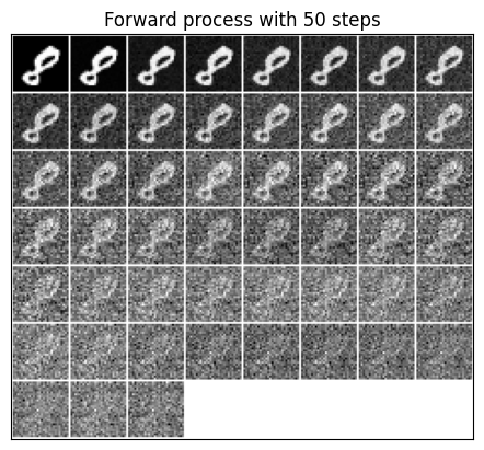
Looks good!

As expected, as we increase $t$ (shown in the grid from left to right, top to bottom) our original image gets increasingly noisy until it is basically just white noise by the last time step $T = 50$.

Reverse Process

Now that we know how to add noise to our data, let’s try to reverse this process and remove noise in order to recover our original image from a noised version of itself.

First, we need to setup the relevant variables from the forward process that generated our noised image $\mathbf{x}_1$from $\mathbf{x}_0$:

# Retrieve the relevant variables from our forward pass
x_1: Float[torch.Tensor, "1 28 28"] = x_1
epsilon_0: Float[torch.Tensor, "1 28 28"] = epsilon_0
alpha_1: float = 1 - beta_1
alpha_bar_1: float = alpha_1
sigma_1: float = np.sqrt(beta_1)
z_1: Float[torch.Tensor, "1 28 28"] = torch.zeros_like(x_0)

Second, we use our diffusion model $\mathbf{\epsilon}_{\theta}$ to estimate the noise that had been added to $\mathbf{x}_1$:

Ideally, you would train a neural network to make this prediction.

However, for this example, let’s just assume that our “model” is able to make a perfect prediction such that $\hat{\epsilon}_0 = \epsilon_0$

# Our diffusion "model" -- we'll circle back on this to get it to actually learn something
def model(x_t, t, true_epsilon, error_scale = 0):
    return true_epsilon + error_scale * torch.randn(x_t.shape)

# Our estimate for the noise (cheat by giving model true epsilon)
epsilon_theta: Float[torch.Tensor, "1 28 28"] = model(x_1, 1, epsilon_0, error_scale=0)

Third, we run the actual diffusion process to remove the noise from $\mathbf{x}_1$ and recover $\mathbf{x}_0$

# Run the reverse process
# => x_t_1 = ....
x_0_hat: Float[torch.Tensor, "1 28 28"] = 1 / np.sqrt(alpha_1) * (x_1 - (1 - alpha_1) / np.sqrt(1 - alpha_bar_1) * epsilon_theta) + sigma_1 * z_1

Let’s see how we did at reversing the diffusion process.

show_grid([ x_0, x_0_hat], title="Original x_0 (left) v. Recovered x_0 (right)")

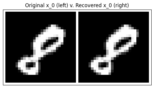
Perfect (as expected)!

Now, let’s see what happens if we have a worse model (i.e. a model that doesn’t perfectly predict the noise that was added at each forward step):

# Our estimate for the noise -- make it slightly off
epsilon_theta: Float[torch.Tensor, "1 28 28"] = model(x_1, 1, epsilon_0, error_scale=1)

# Run the reverse process
x_0_hat: Float[torch.Tensor, "1 28 28"] = 1 / np.sqrt(alpha_1) * (x_1 - (1 - alpha_1) / np.sqrt(1 - alpha_bar_1) * epsilon_theta) + sigma_1 * z_1

# Show denoised image
show_grid([ x_0, x_0_hat], title="Original x_0 (left) v. Recovered x_0 (right)")

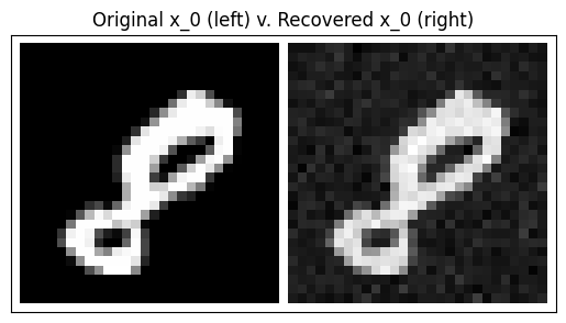
As you can see, the worse our estimate for $\mathbf{\epsilon}_0$, the more inacurrate our recovered image is.

Training the model

Now that we understand how the forward / reverse processes work, let’s train a model to learn the reverse process.

The core training algorithm that we will be implementing is the following:

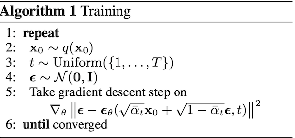
Training algorithm from Ho et al. 2020. Credit: https://arxiv.org/pdf/2006.11239.pdf

First, let’s setup our diffusion model’s hyperparameters.

Again, they are:

# Hyperparams for diffusion model
T: int = 50 # number of steps
betas: Float[np.ndarray, "T"] = torch.linspace(1e-4, 1e-1, T)
alphas: Float[np.ndarray, "T"] = 1 - betas
alpha_bars: Float[torch.Tensor, "T"] = torch.Tensor(np.cumprod(alphas))
sigmas: Float[torch.Tensor, "T"] = torch.sqrt(betas)

# General training stuff
N_EPOCHS: int = 5
LOGGING_STEPS: int = 5

Second, let’s define the model $\mathbf{\epsilon_{\theta}}$ that we will use to predict $\mathbf{\epsilon}_t$ given $\mathbf{x}_t$ and $t$.

This could be any arbitrary model, but for our purposes we will use a slightly modified PixelCNN model, as was used in Ho et al. 2020.

Note the line of code from model import Model. This model is imported from this file here, and was originally taken (with minimal modifications) from this Github repo. To run this notebook yourself, you will need to download the model.py file and place it in the same directory as this notebook.

# Setup PixelCNN model
config = {
    'data': {
        'image_size': 28,
    },
    'model': {
        'type': "simple",
        'in_channels': 1,
        'out_ch': 1,
        'ch': 128,
        'ch_mult': [1, 2, 2,],
        'num_res_blocks': 2,
        'attn_resolutions': [1, ],
        'dropout': 0.1,
        'resamp_with_conv': True,
    },
    'diffusion': {
        'num_diffusion_timesteps': T,
    },
    'runner' : {
        'n_epochs' : N_EPOCHS,
        'logging_steps' : LOGGING_STEPS,
    }
}
def dict2namespace(config):
    namespace = argparse.Namespace()
    for key, value in config.items():
        if isinstance(value, dict):
            new_value = dict2namespace(value)
        else:
            new_value = value
        setattr(namespace, key, new_value)
    return namespace
config = dict2namespace(config)

# Create diffusion model
from model import Model
model = Model(config)
optimizer = torch.optim.Adam(model.parameters(), lr=2e-4)

Now let’s write our actual training loop.

The inner loop of the code below works as follows.

1. Sample an example $\mathbf{x}_0$ from our training dataset $q(\mathbf{x}_0)$.
   • As an equation: $\mathbf{x}_0 \sim q(\mathbf{x}_0)$.
   • Note that we actually sample several $\mathbf{x}_0$ at once to create a batch of inputs to simultaneously feed through our model. This is denoted by the variable B in the below code, which stands for “batch size”
   • For clarity, I will ignore this batch dimension in the following steps, but just keep in mind that all of these steps are actually being done B times in parallel.
2. Sample a timestep $t$ uniformly at random. This is how many timesteps of noise we will apply to our $\mathbf{x}_0$.
   • As an equation: $t \sim \text{Uniform}(0, T)$.
3. Sample how much noise we add to $\mathbf{x}_0$ at each timestep $t$.
   • As an equation: $\mathbf{\epsilon} \sim N(0, \textbf{I})$.
4. Run the forward process to generate $\mathbf{x}_t \sim q(\mathbf{x}_t \vert \mathbf{x}_0)$.
5. Have our diffusion model (PixelCNN) predict how much noise was added to $\mathbf{x}_t$.
   • As an equation: $\hat{\epsilon} = \mathbf{\epsilon}_{\theta}(\mathbf{x}_t, t)$, where $\theta$ represents the parameters of the PixelCNN deep learning model and $\mathbf{\epsilon}_{\theta}$ is our diffusion model.
6. Calculate our loss, which is the squared error between our predicted noise $\hat{\epsilon}$ and the true noise $\epsilon$.
   • As an equation: $\vert\vert \mathbf{\epsilon} - \hat{\mathbf{\epsilon}}\vert\vert^2$
   • We can rewrite this to match the notation in Ho et al. 2020’s training algorithm as:

1. Take a gradient descent step on the gradient of our loss via PyTorch’s built-in loss.backward() autograd function.
   • As an equation: $ \nabla_{\theta} \vert\vert \mathbf{\epsilon} - \mathbf{\epsilon_{\theta}}(\sqrt{\bar{\alpha}_t} \mathbf{x}_0 + \sqrt{1 - \bar{\alpha_t}} \mathbf{\epsilon}, t) \vert\vert^2$

def train(model, config, optimizer, trainloader, T: int, alpha_bars):
    '''Train diffusion model.'''
    n_epochs: int = config.runner.n_epochs
    logging_steps: int = config.runner.logging_steps
    
    losses: List[float] = []
    model.train()
    for epoch in range(n_epochs):
        train_loss: float = 0.0

        start_time = time.time()
        for batch_idx, (x_0, _) in enumerate(trainloader):
            B: int = x_0.shape[0] # batch size
            # Sample x_0 ~ q(x_0)
            x_0: Float[torch.Tensor, "B 1 28 28"] = x_0.to(model.device)
            # Sample t ~ U(0, T)
            t: Float[torch.Tensor, "B"] = torch.randint(0, T, (B,))
            # Sample e ~ N(0, I)
            epsilon: Float[torch.Tensor, "B 1 28 28"] = torch.randn(x_0.shape, device=model.device)
            # Sample x_t ~ q(x_t | x_0) = sqrt(alpha_bar) x_0 + sqrt(1 - alpha_bar) e
            x_0_coef = torch.sqrt(alpha_bars[t]).reshape(-1, 1, 1, 1).to(model.device)
            epsilon_coef = torch.sqrt(1 - alpha_bars[t]).reshape(-1, 1, 1, 1).to(model.device)
            x_t: Float[torch.Tensor, "B 1 28 28"] = x_0_coef * x_0 + epsilon_coef * epsilon
            # Predict epsilon_theta = f(x_t, t)
            epsilon_theta: Float[torch.Tensor, "B 1 28 28"] = model(x_t, t.to(model.device))
            # Calculate loss
            loss: float = torch.sum((epsilon - epsilon_theta)**2)
            # Backprop gradient
            loss.backward()
            optimizer.step()
            optimizer.zero_grad()
            
            # Logging
            losses.append(loss.item())
            train_loss += loss.item()
            if (batch_idx + 1) % logging_steps == 0 : 
                deno = logging_steps * B
                print(
                    'Loss over last {} batches: {:.4f} | Time (s): {:.4f}'.format(
                    logging_steps, (train_loss / deno), (time.time() - start_time))
                )
                train_loss = 0.0
                start_time = time.time()

    return model, losses

Let’s train our model for N_EPOCHS iterations. I’m using a Macbook, so we’ll use the MPS system for training.

# Train model
model = model.to('mps')
model, losses = train(model, config, optimizer, train_dataloader, T, alpha_bars)
torch.save(model.state_dict(), f'model.pt')

This model ran for 5 epochs (18750 total batches) at an average rate of 0.43s per batch, for a total training time of about 2 hours and 15 minutes.

Let’s see what the per-batch loss curve looks like:

plt.plot(losses)
plt.show()

[<matplotlib.lines.Line2D at 0x16d9a4990>]

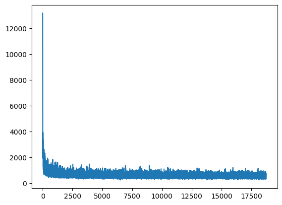
As you can see, I did a terrible job initializing this model (as seen in the huge jump in the first ~100 batches), and the model essentially stopped learning within the first 5000-ish steps.

Clearly, we can spend more time tuning hyperparameters for both our diffusion process (i.e. setting $T$ to a larger number than 50) and PixelCNN model to get better results.

Anyway, the point of this exercise was simply to implement a basic model, so let’s see how we did.

Inference

Now that we have a trained diffusion model, we can run inference on it to generate new data that looks like it came from our training dataset, i.e. MNIST.

The algorithm we’re implementing, taken directly from Ho et al. 2020, is as follows:

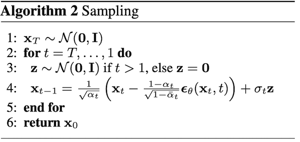Inference (i.e. “sampling”) algorithm, taken from Ho et al. 2020. Credit: https://arxiv.org/pdf/2006.11239.pdf

Below, I wrote a function called inference() which translates this mathematical algorithm into Python code.

The code works as follows. Again, remember that everything is actually batched so that we can generate B unique outputs at once. You can think of it as running the below code B times in parallel.

1. Sample random Gaussian noise.
   • As an equation: $\mathbf{x}_T \sim N(0, \mathbf{I})$
2. For timesteps $t = T, T-1, …, 1$:
   1. If $t > 1$, sample random Gaussian noise to add to our denoised image. Otherwise, if $t = 0$ then we’re at the last step of our reverse process, so don’t add any noise to our denoised image.
      • As an equation: $\mathbf{z} \sim N(0, \mathbf{I})$ if $t > 1$ else $\mathbf{z} = \mathbf{0}$
   2. Run the reverse process: $\mathbf{x}_{t-1} \sim p_{\theta}(x_{t-1} \vert x_t)$
      • As an equation: $\mathbf{x}_{t-1} = \frac{1}{\sqrt{\alpha_{t}}} ( \mathbf{x}_t + \frac{1 - \alpha_t}{\sqrt{1 - \bar{\alpha}_t}} \mathbf{\epsilon}_{\theta}(\mathbf{x}_t, t) ) + \sigma_t \mathbf{z}$
3. Return the denoised image $\mathbf{x}_0$.

def inference(model, config, n_samples: int, T: int, alphas, alpha_bars, sigmas, seed: int = 1) -> Float[torch.Tensor, "n_samples T 1 28 28"]:
    '''Generate images from diffusion model.'''
    model.eval()
    torch.manual_seed(seed)
    # Dimensions
    n_channels: int = config.model.in_channels # 1 for grayscale
    H, W = config.data.image_size, config.data.image_size # 28 pixels
    # x_T \sim N(0, I)
    x_T: Float[torch.Tensor, "n_samples 28 28"] = torch.randn((n_samples, n_channels, W, W))
    # For t = T ... 1
    x_t = x_T
    x_ts = [] # save image as diffusion occurs
    for t in tqdm(range(T-1, -1, -1)):
        # z \sim N(0, I) if t > 1 else z = 0
        z: Float[torch.Tensor, "n_samples 1 28 28"] = torch.randn(x_t.shape) if t > 1 else torch.zeros_like(x_t)
        # Setup terms for x_t-1
        t_vector: Float[torch.Tensor, "n_samples"] = torch.fill(torch.zeros((n_samples,)), t)
        epsilon_theta: Float[torch.Tensor, "n_samples 1 28 28"] = model(x_t.to(model.device), t_vector.to(model.device)).to('cpu')
        # x_t-1 = (1 / sqrt(alpha_t)) * (x_t - (1 - alpha_t) / (sqrt(1 - alpha_bar_t)) * epsilon_theta(x_t, t)) + sigma_t * z
        x_t_1: Float[torch.Tensor, "n_samples 1 28 28"]  = (
            1 / torch.sqrt(alphas[t]) * (x_t - (1 - alphas[t]) / torch.sqrt(1 - alpha_bars[t]) * epsilon_theta)
            + sigmas[t] * z
        )
        x_ts.append(x_t)
        x_t = x_t_1
    return torch.stack(x_ts).transpose(0, 1)

Now, let’s reload our trained diffusion model and generate an image from it!

# Load model
model = Model(config)
model.load_state_dict(torch.load(f"model.pt"))
model = model.to('mps')

sampled_images: Float[torch.Tensor, "n_samples T 1 28 28"] = inference(model, config, 2, T, alphas, alpha_bars, sigmas, seed=6)
for sample in sampled_images:
    show_grid(sample, title=f"Sampled Image from Diffusion Model")
    plt.show()

100%|██████████| 50/50 [00:04<00:00, 10.24it/s]

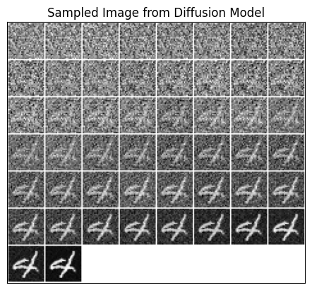
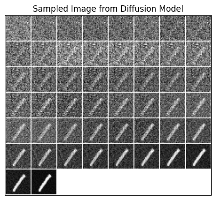
Not bad!

Ignoring the cherrypicked random seed for a second, it looks like we were able to successfully generate a 4 and a 1 from pure noise.

But how do we know that the model isn’t simply regurgitating training data that it’s memorized, i.e. overfitting?

We can check this by finding the closest training example to each of our generated images, then visually inspect how similar they are. We will use the Euclidean distance to measure how “close” two images are to each other.

# Find closest image to x_0 in our training dataset
for x_0 in sampled_images[:,-1,...]:
    x_0 = x_0.squeeze(1)

    # Rescale to be between [-1, 1]
    x_0 = 2 * (x_0 - x_0.min()) / (x_0.max() - x_0.min()) - 1
    train_min = train_dataset.data.view(train_dataset.data.shape[0], -1).min(dim=1, keepdim=True)[0].unsqueeze(2)
    train_max = train_dataset.data.view(train_dataset.data.shape[0], -1).max(dim=1, keepdim=True)[0].unsqueeze(2)
    train_data = 2 * (train_dataset.data - train_min) / (train_max - train_min) - 1

    # Find training image with minimal Euclidean distance from x_0
    distances = torch.sum((train_data - x_0) ** 2, dim=(1, 2,))
    show_grid([ train_dataset[torch.argmin(distances)][0], x_0 ], title=f"Closest Image in Training Set (left) to Generated Image (right)")

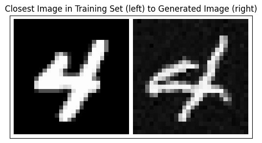
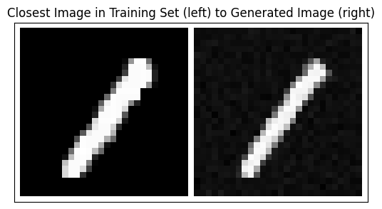
While the images are pretty close, they are clearly different (especially the 4). Thus, we can have more confidence that our model actually learned something about how to generate new MNIST images from pure noise.

Conclusion

That brings me to the end of this tutorial.

Hopefully you learned something about diffusion models along the way.

Again, please note that I am not an expert by any means – I wrote this tutorial as a way to learn about diffusion models myself, and I’m sure there are mistakes in my explanations. If you find any, please let me know!

References

• Great tutorial on variational inference: https://mpatacchiola.github.io/blog/2021/01/25/intro-variational-inference.html
• Ho et al. 2020 original paper: https://arxiv.org/pdf/2006.11239.pdf
• More mathy tutorial: https://lilianweng.github.io/posts/2021-07-11-diffusion-models/